DRL Temporal-Difference Mothods

from IPython.display import Image
Image(filename='./images/1-0-0-1_opening.jpg')

Lesson 1-5: Temporal-Difference Methods

This lesson covers material in Chapter 6 (especially 6.1-6.6) of the Sutton’s textbook.

Real life is far from an episodic task and it requires its agents, it requires us to constantly make decisions all day everyday. We get no break with our interaction with the world. Remember that Monte Carlo learning needed those breaks, it needed the episode to end so that the return could be calculated, and then used as an estimate for the action values. So, we’ll need to come up with something else if we want to deal with more realistic learning in a real world setting.

So, the main idea is this, if an agent is playing chess, instead of waiting until the end of an episode to see if it’s won the game or not, it will at every move be able to estimate the probability that it’s winning the game, or a self-driving car at every turn will be able to estimate if it’s likely to crash, and if necessary, amend its strategy to avoid disaster. To emphasize, the Monte Carlo approach would have this car crash every time it wants to learn anything, and this is too expensive and also quite dangerous.

TD learning will solve these problems. Instead of waiting to update values when the interaction ends, it will amend its predictions at every step, and you’ll be able to use it to solve both continuous and episodic tasks.

1-5-1 : Review: MC Control Methods

you learned about the control problem in reinforcement learning and implemented some Monte Carlo (MC) control methods.

Control Problem: Estimate the optimal policy.

In this lesson, you will learn several techniques for Temporal-Difference (TD) control.

from IPython.display import Image
Image(filename='./images/1-5-1-1_constant-α_MC_control_algorithm_alternates_between_policy_evaluation_and_policy_improvement.png')

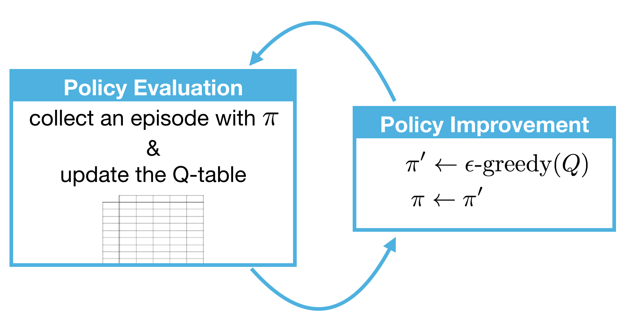
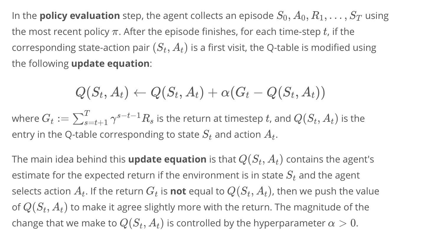
Remember that the constant-α MC control algorithm alternates between policy evaluation and policy improvement steps to recover the optimal policy π∗.

from IPython.display import Image
Image(filename='./images/1-5-1-2_constant-α_MC_control_algorithm_policy_update_equation.png')

Quiz

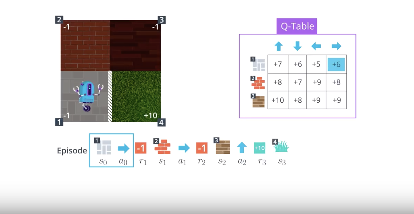
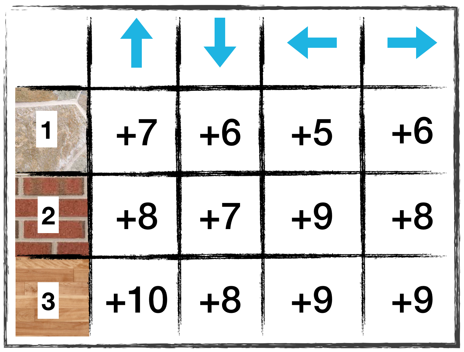
Say that an agent is learning to navigate the gridworld described in the above videos. Suppose the agent is using Constant-α MC control in its search for the optimal policy, with α=0.1. At the end of the 99th episode, the Q-table has the following values:

from IPython.display import Image
Image(filename='./images/1-5-1-3_constant-α_MC_control_algorithm_quiz_q-table.png')

from IPython.display import Image
Image(filename='./images/1-5-1-4_constant-α_MC_control_algorithm_quiz_1000th_episode.png')

What is the new value for the entry in the Q-table corresponding to state 1 and action right?

• 6
• 6.1
• 6.16
• 6.2
• 7
• 9

1-5-2 : TD Control: Sarsa

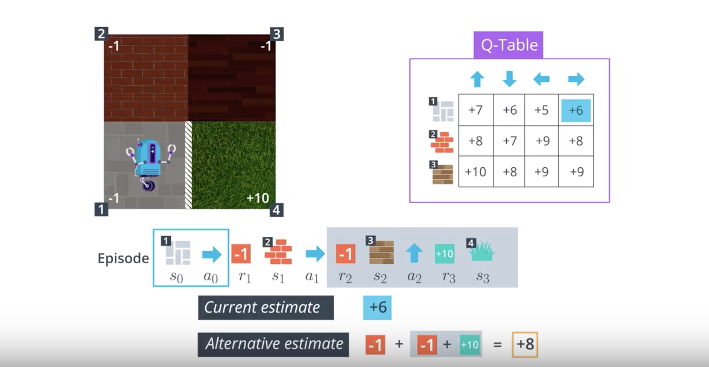
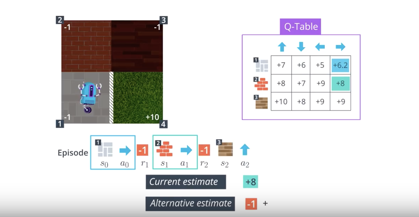
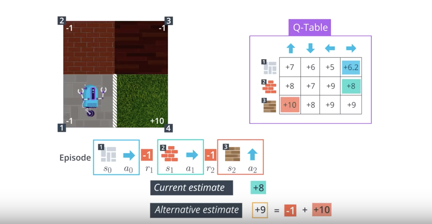
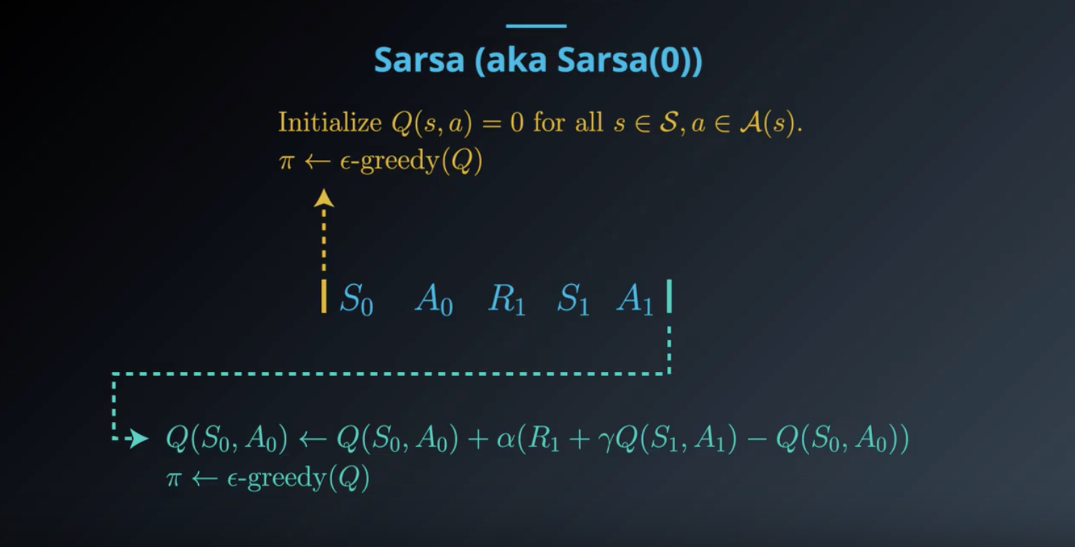
Monte Carlo (MC) control methods require us to complete an entire episode of interaction before updating the Q-table. Temporal Difference (TD) methods will instead update the Q-table after every time step.

from IPython.display import Image
Image(filename='./images/1-5-2-1_sarsa0_step1.png')

from IPython.display import Image
Image(filename='./images/1-5-2-2_sarsa0_alternative_estimate_by_mc_control.png')

from IPython.display import Image
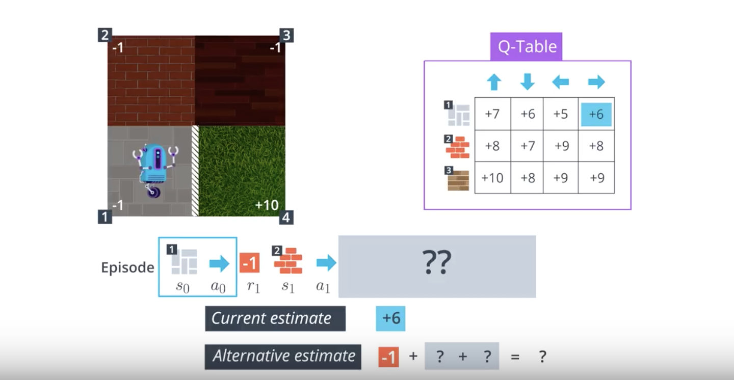
Image(filename='./images/1-5-2-3_sarsa0_step2.png')

from IPython.display import Image
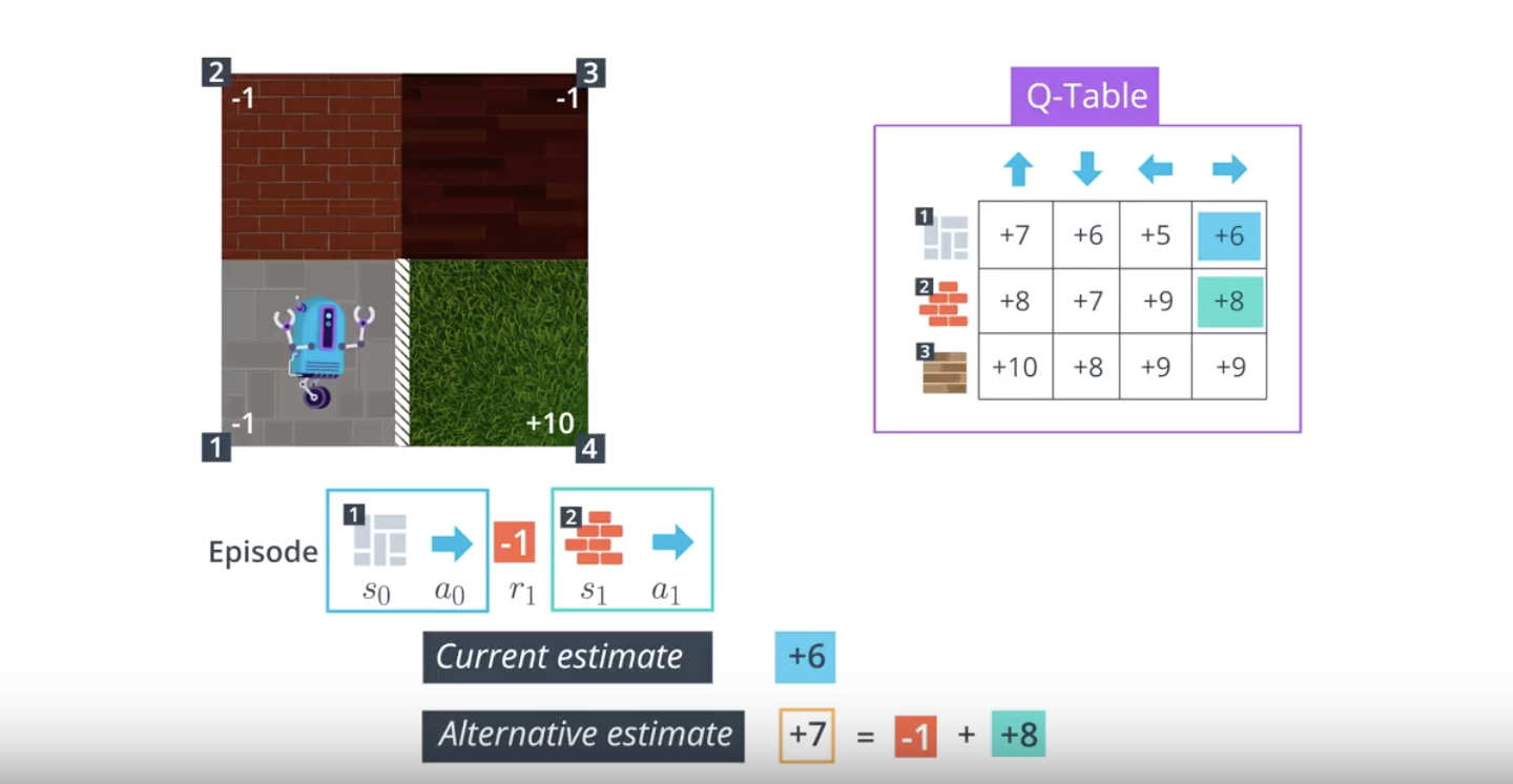
Image(filename='./images/1-5-2-4_sarsa0_step3.png')

from IPython.display import Image
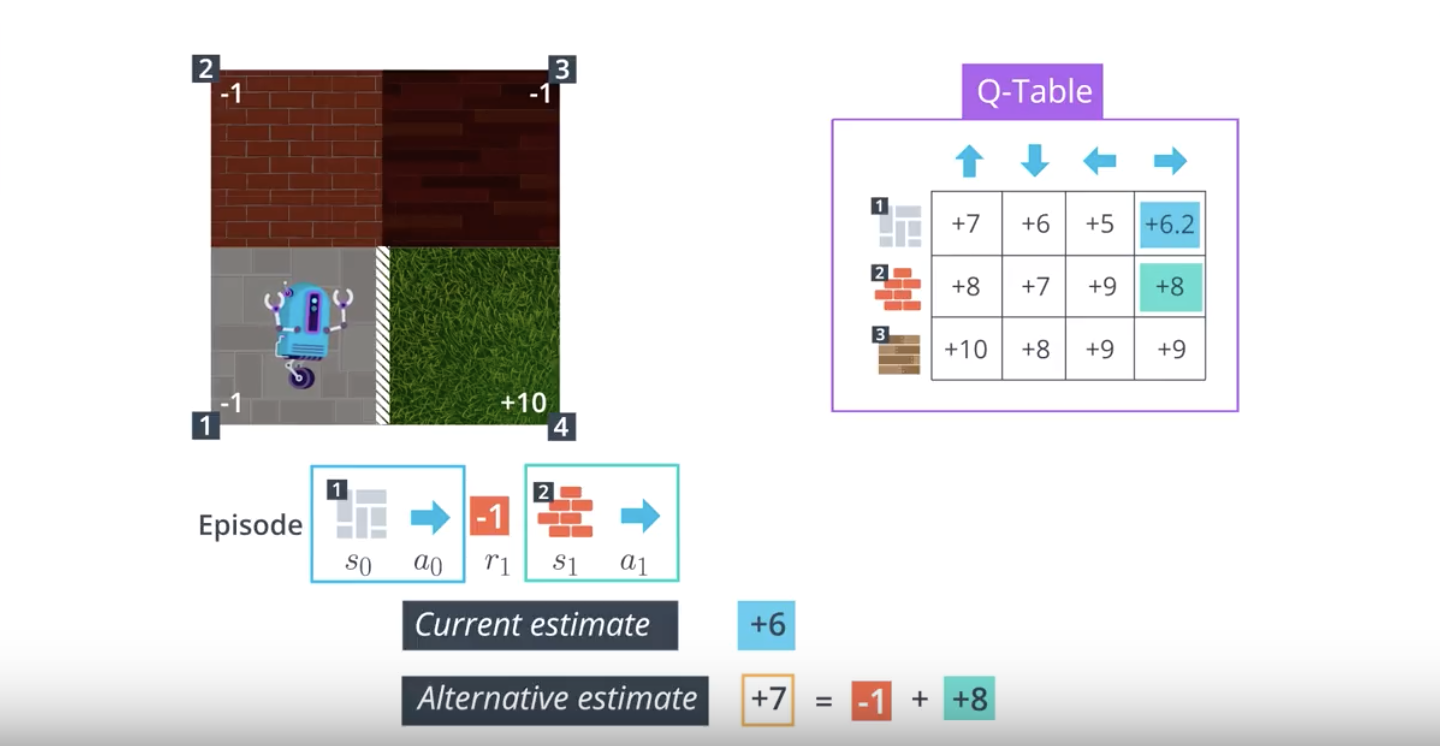
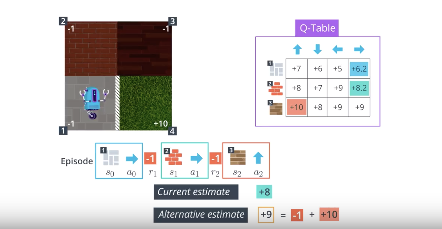
Image(filename='./images/1-5-2-5_sarsa0_step4.png')

from IPython.display import Image
Image(filename='./images/1-5-2-6_sarsa0_step5.png')

from IPython.display import Image
Image(filename='./images/1-5-2-7_sarsa0_step6.png')

from IPython.display import Image
Image(filename='./images/1-5-2-8_sarsa0_step7.png')

from IPython.display import Image
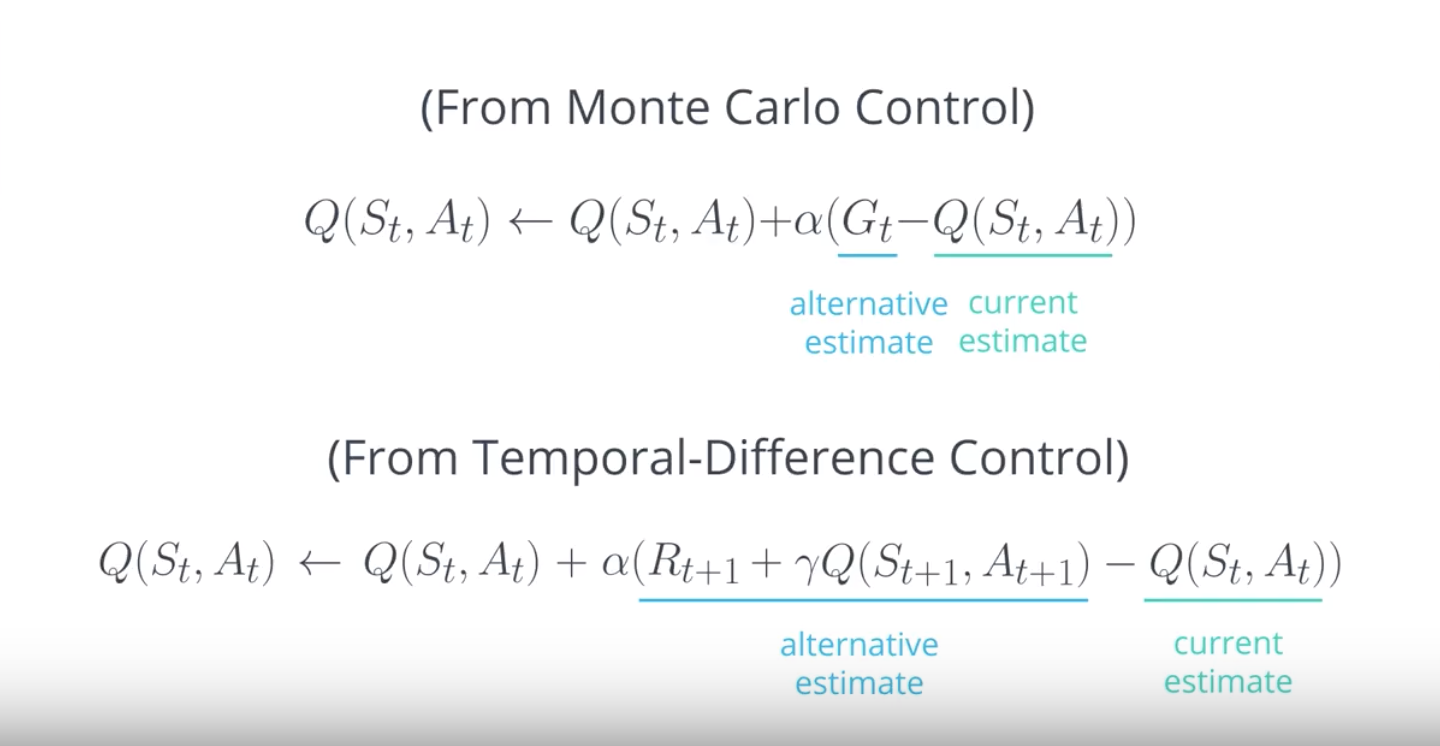
Image(filename='./images/1-5-2-9_sarsa0_td_control_equation.png')

from IPython.display import Image
Image(filename='./images/1-5-2-10_sarsa0_td_control_explanation.png')

from IPython.display import Image
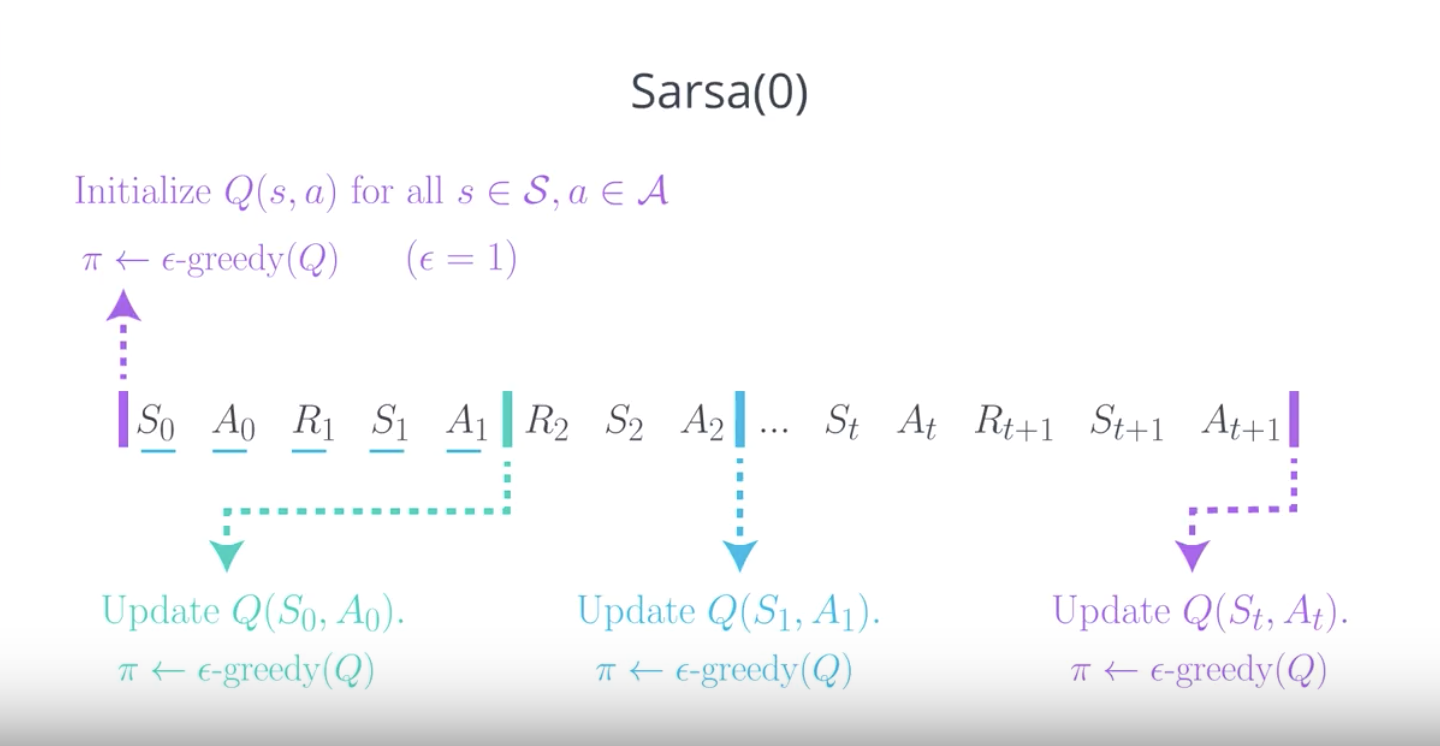
Image(filename='./images/1-5-2-11_sarsa0_pseudocode.png')

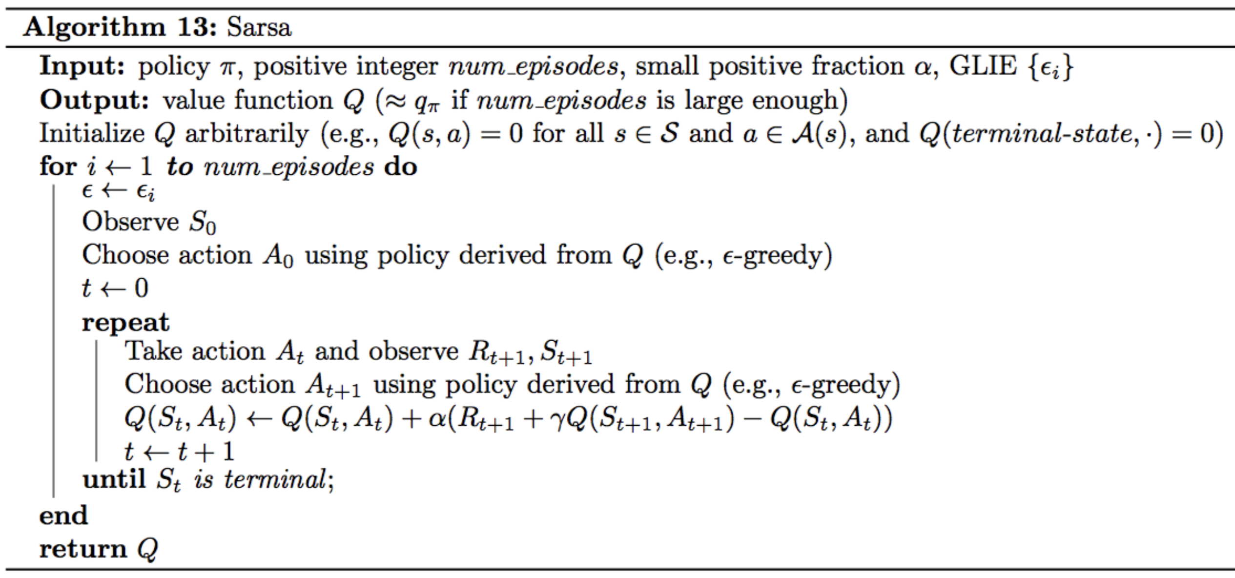
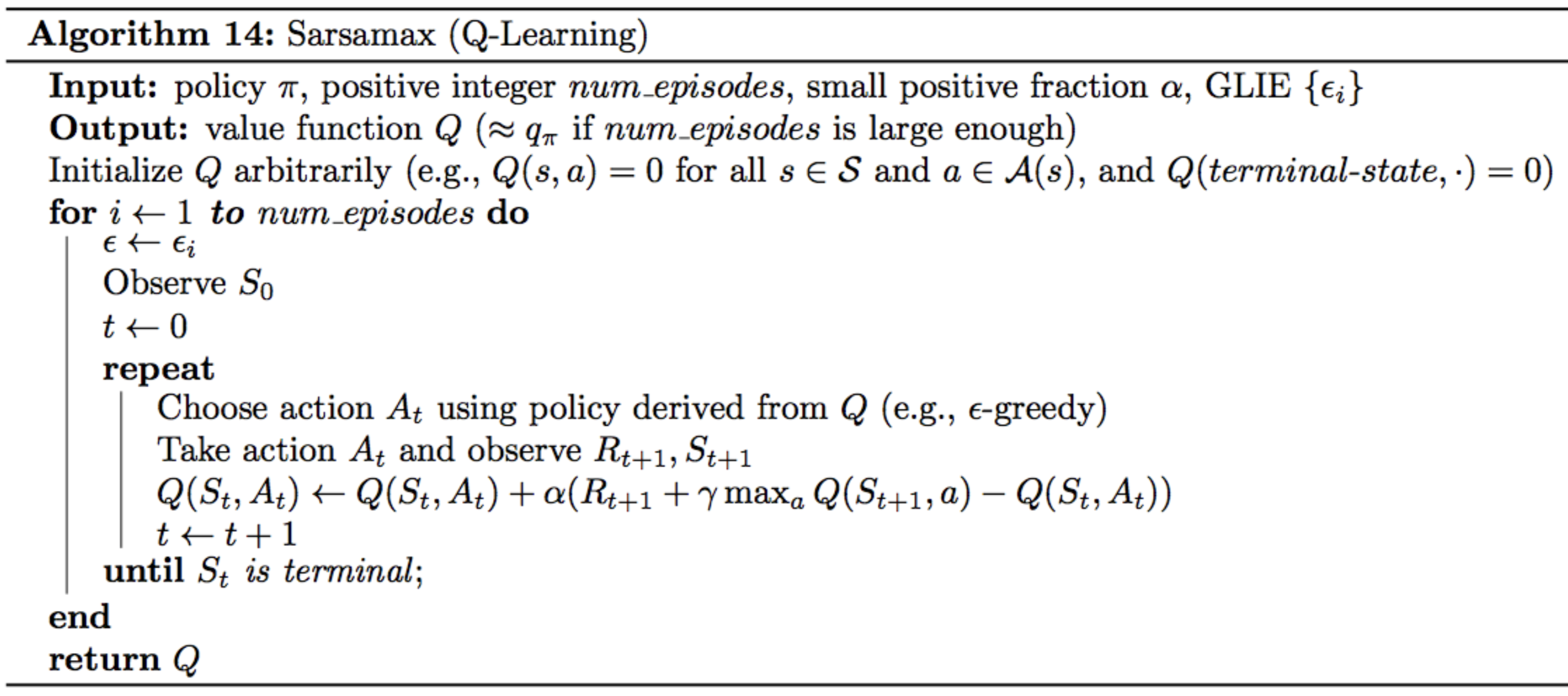
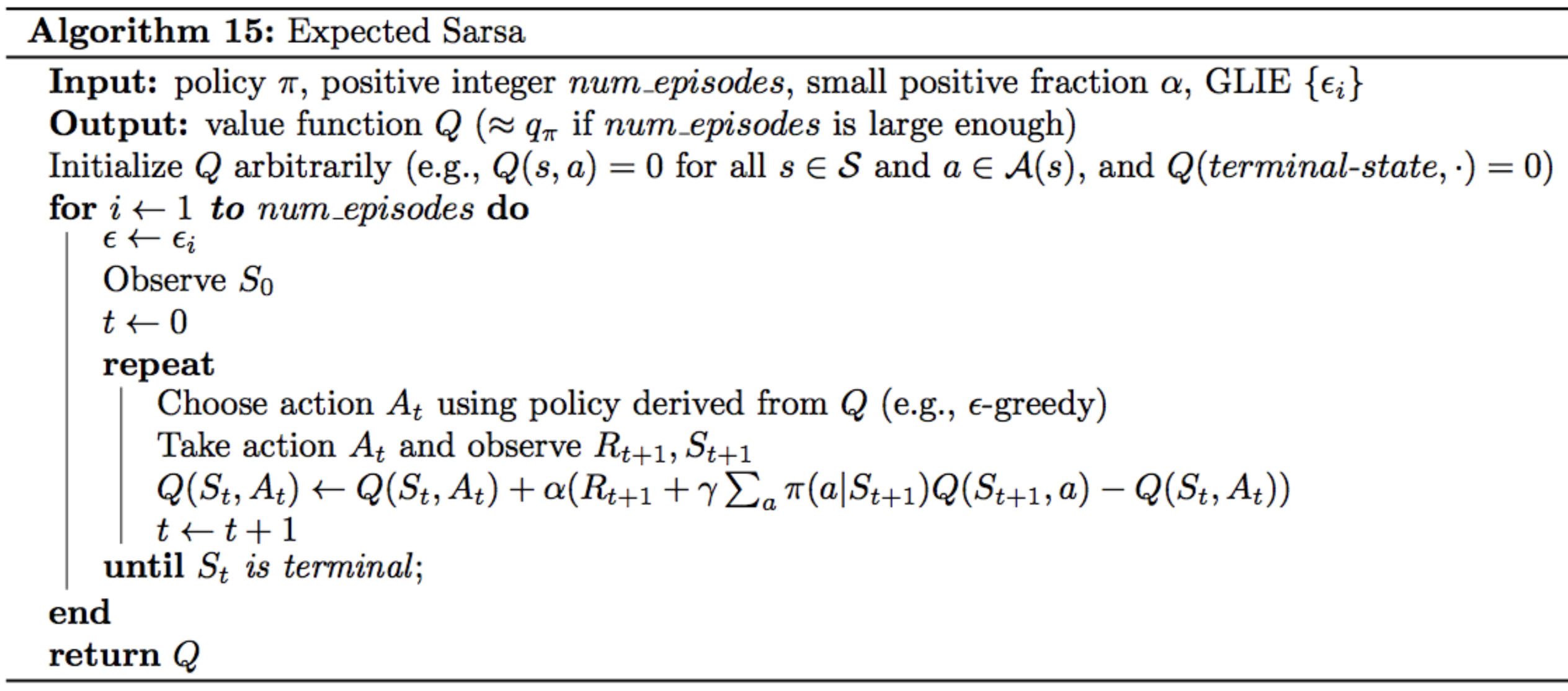
In the algorithm, the number of episodes the agent collects is equal to num_episodes. For every time step t≥0, the agent:

• takes the action At(from the current state St) that is ϵ-greedy with respect to the Q-table, receives the reward Rt+1 and next state St+1,
• chooses the next action At+1(from the next state St+1) that is ϵ-greedy with respect to the Q-table,
• uses the information in the tuple (St, At, Rt+1, St+1, At+1) to update the entry Q(St,At) in the Q-table corresponding to the current state St and the action At.

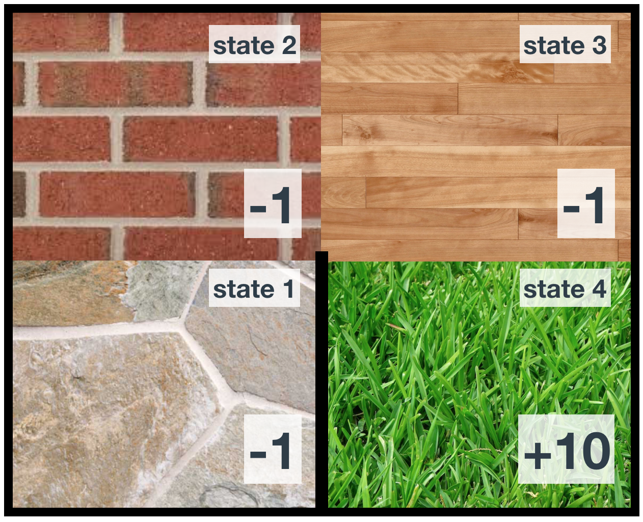
Quiz: Sarsa

from IPython.display import Image
Image(filename='./images/1-5-2-12_sarsa0_quiz_environment.png')

from IPython.display import Image
Image(filename='./images/1-5-2-13_sarsa0_quiz_q-table.png')

from IPython.display import Image
Image(filename='./images/1-5-2-14_sarsa0_quiz_100th-episode.png')

QUESTION 1 OF 2

Which entry in the Q-table is updated?

(Suppose the agent is using Sarsa in its search for the optimal policy, with α=0.1.)

1. The entry corresponding to state 1 and action left.
2. The entry corresponding to state 2 and action left.
3. The entry corresponding to state 1 and action right.
4. The entry corresponding to state 2 and action right.

QUESTION 2 OF 2

What is the new value in the Q-table corresponding to the state-action pair you selected in the answer to the question above?

(Suppose that when selecting the actions for the first two timesteps in the 100th episode, the agent was following the epsilon-greedy policy with respect to the Q-table, with epsilon = 0.4.)

1. 6
2. 6.1
3. 6.16
4. 6.2
5. 7
6. 9

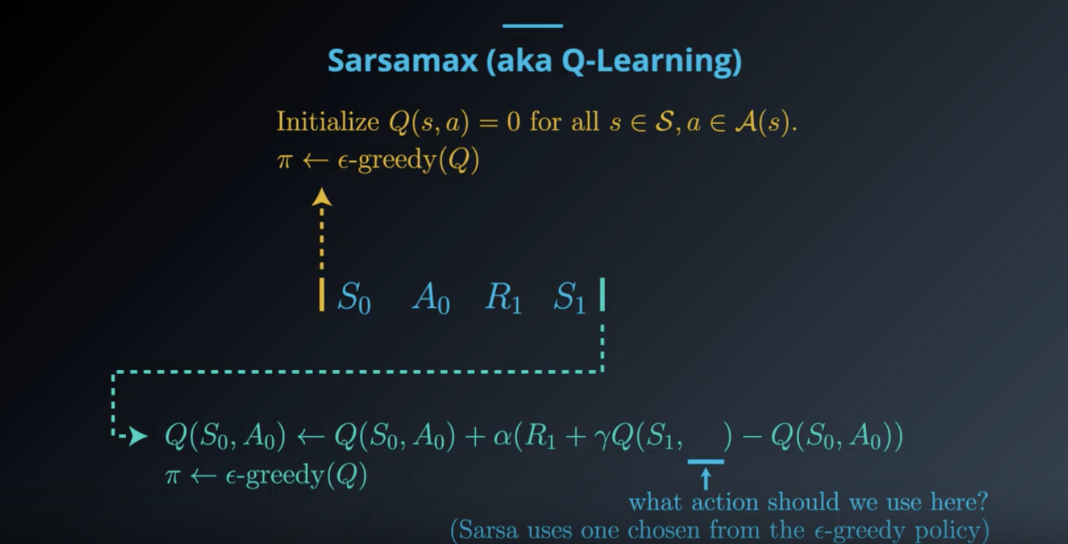
1-5-3 : TD Control: Q-Learning

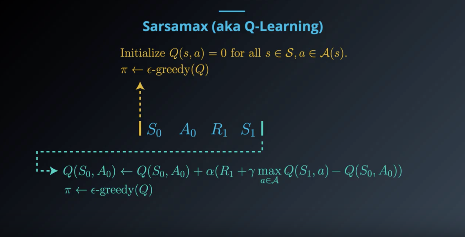
Q-Learning (or Sarsamax), a second method for TD control.

from IPython.display import Image
Image(filename='./images/1-5-3-1_sarsamax_the_control_problem.png')

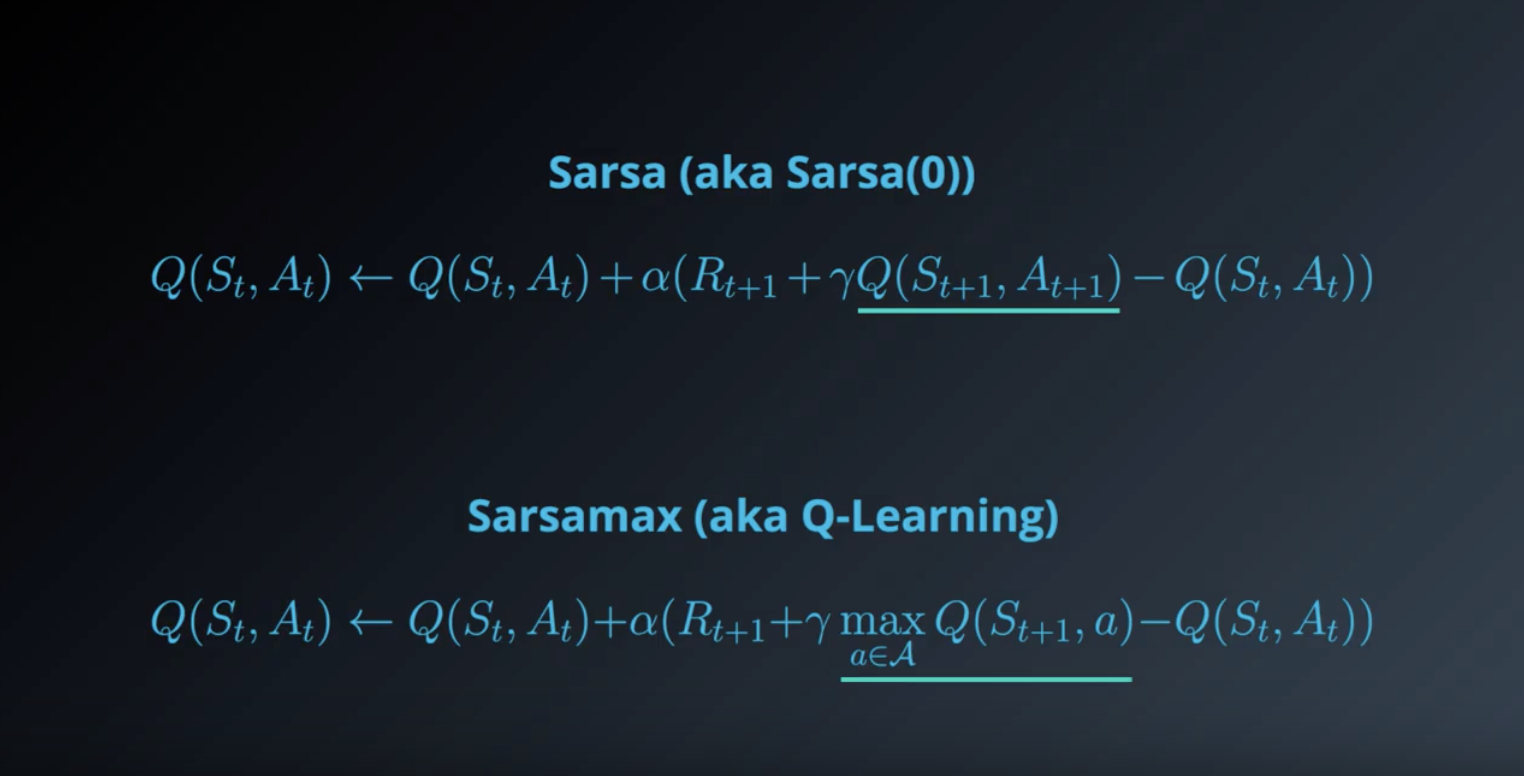
from IPython.display import Image
Image(filename='./images/1-5-3-2_sarsamax_sarsa-zero.png')

from IPython.display import Image
Image(filename='./images/1-5-3-3_sarsamax_step1.png')

from IPython.display import Image
Image(filename='./images/1-5-3-3_sarsamax_step1.png')

from IPython.display import Image
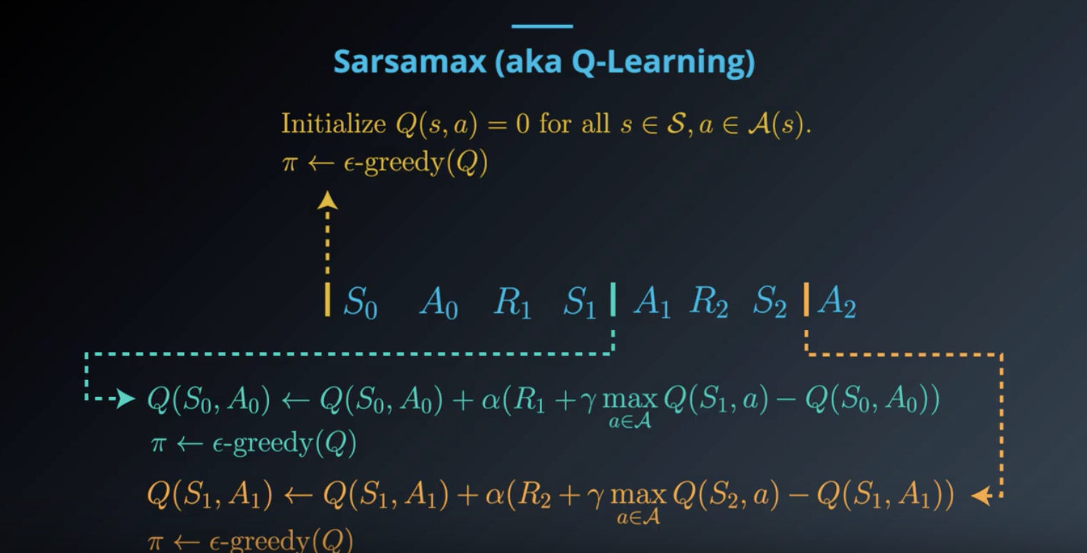
Image(filename='./images/1-5-3-4_sarsamax_step2.png')

from IPython.display import Image
Image(filename='./images/1-5-3-5_sarsamax_step3.png')

from IPython.display import Image
Image(filename='./images/1-5-3-6_sarsamax_equation.png')

from IPython.display import Image
Image(filename='./images/1-5-3-7_sarsamax_pseudocode.png')

Check out this (optional) research paper to read the proof that Q-Learning (or Sarsamax) converges.

Quiz: Q-Learning

from IPython.display import Image
Image(filename='./images/1-5-3-8_sarsamax_quiz_environment.png')

from IPython.display import Image
Image(filename='./images/1-5-3-9_sarsamax_quiz_q-table_at_99th_episode.png')

from IPython.display import Image
Image(filename='./images/1-5-3-10_sarsamax_quiz_100th-episode.png')

QUESTION 1 OF 2

Which entry in the Q-table is updated?

(Suppose the agent is using Q-Learning in its search for the optimal policy, with α=0.1.)

1. The entry corresponding to state 1 and action left.
2. The entry corresponding to state 2 and action left.
3. The entry corresponding to state 1 and action right.
4. The entry corresponding to state 2 and action right.

QUESTION 2 OF 2

What is the new value in the Q-table corresponding to the state-action pair you selected in the answer to the question above?

(Suppose that when selecting the actions for the first two timesteps in the 100th episode, the agent was following the epsilon-greedy policy with respect to the Q-table, with epsilon = 0.4.)

1. 6
2. 6.1
3. 6.16
4. 6.2
5. 7
6. 9

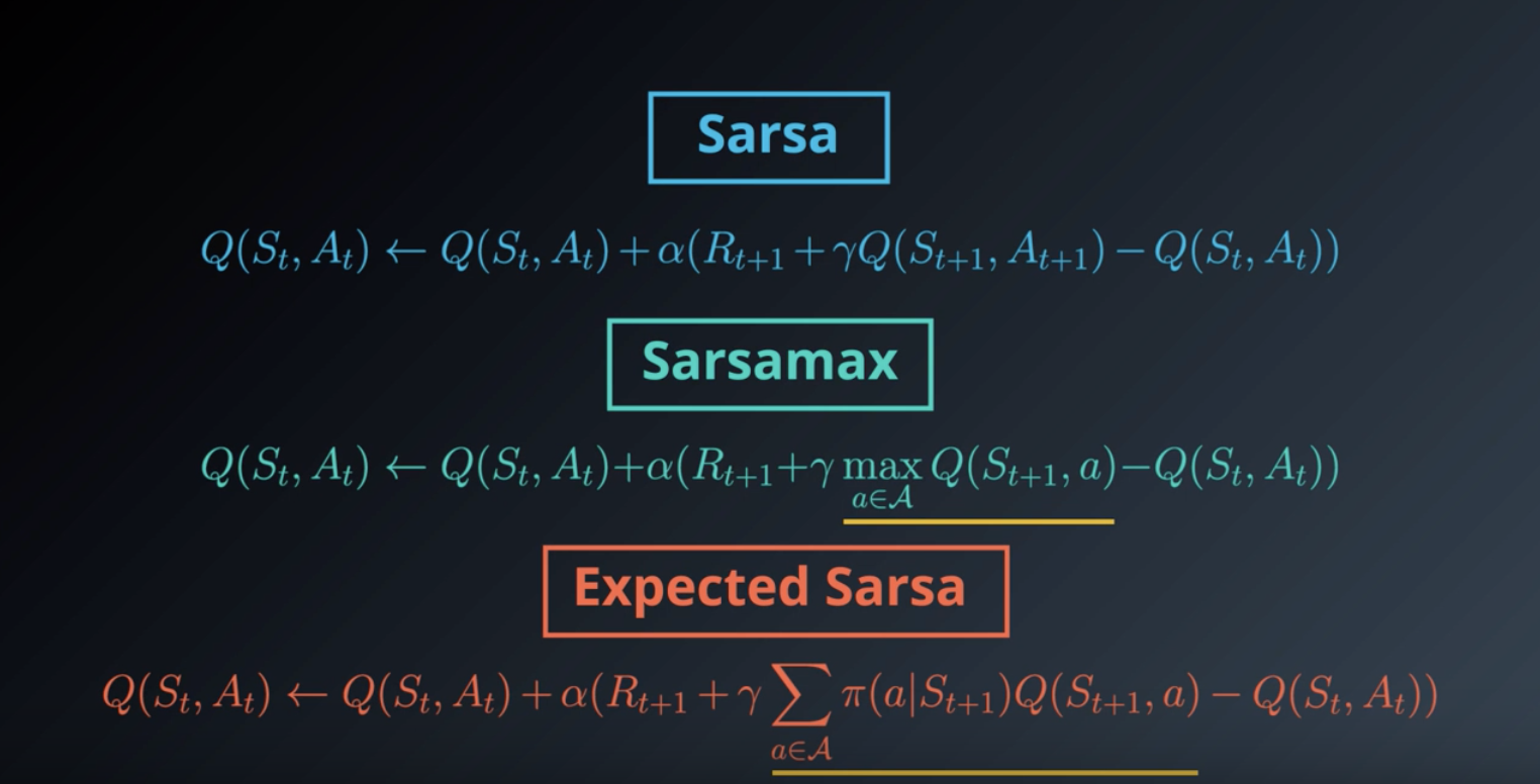
1-5-4 : TD Control: Expected Sarsa

Expected Sarsa, a third method for TD control.

from IPython.display import Image
Image(filename='./images/1-5-4-1_expected-sarsa.png')

from IPython.display import Image
Image(filename='./images/1-5-4-2_expected-sarsa_pseudocode.png')

Check out this (optional) research paper to learn more about Expected Sarsa.

Quiz: Expected Sarsa

from IPython.display import Image
Image(filename='./images/1-5-4-3_expected-sarsa_quiz_environment.png')

from IPython.display import Image
Image(filename='./images/1-5-4-4_expected-sarsa_quiz_q-table_at_99th_episode.png')

from IPython.display import Image
Image(filename='./images/1-5-4-5_expected-sarsa_quiz_100th-episode.png')

QUESTION 1 OF 2

Which entry in the Q-table is updated?

(Suppose the agent is using Expected Sarsa in its search for the optimal policy, with α=0.1.)

1. The entry corresponding to state 1 and action left.
2. The entry corresponding to state 2 and action left.
3. The entry corresponding to state 1 and action right.
4. The entry corresponding to state 2 and action right.

QUESTION 2 OF 2

What is the new value in the Q-table corresponding to the state-action pair you selected in the answer to the question above?

(Suppose that when selecting the actions for the first two timesteps in the 100th episode, the agent was following the epsilon-greedy policy with respect to the Q-table, with epsilon = 0.4.)

1. 6
2. 6.1
3. 6.16
4. 6.2
5. 7
6. 9

1-5-5 : TD Control: Theory and Practice

Greedy in the Limit with Infinite Exploration (GLIE)

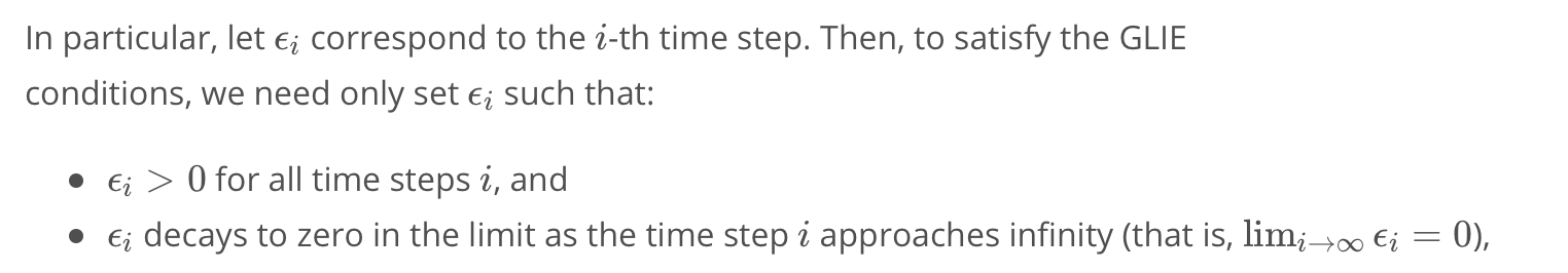
The Greedy in the Limit with Infinite Exploration (GLIE) conditions were introduced in the previous lesson, when we learned about MC control. There are many ways to satisfy the GLIE conditions, all of which involve gradually decaying the value of ϵ when constructing ϵ-greedy policies.

from IPython.display import Image
Image(filename='./images/1-5-5-1_TD Control_Theory-and-Practice.png')

In Theory

All of the TD control algorithms we have examined (Sarsa, Sarsamax, Expected Sarsa) are guaranteed to converge to the optimal action-value function q∗, as long as the step-size parameter α is sufficiently small, and the GLIE conditions are met.

from IPython.display import Image
Image(filename='./images/1-5-5-2_TD Control_Theory-and-Practice.png')

In Practice

In practice, it is common to completely ignore the GLIE conditions and still recover an optimal policy.

Optimism

You have learned that for any TD control method, you must begin by initializing the values in the Q-table. It has been shown that initializing the estimates to large values can improve performance. For instance, if all of the possible rewards that can be received by the agent are negative, then initializing every estimate in the Q-table to zeros is a good technique. In this case, we refer to the initialized Q-table as optimistic, since the action-value estimates are guaranteed to be larger than the true action values.

1-5-6 : Analyzing Performance

You’ve learned about three different TD control methods in this lesson. So, what do they have in common, and how are they different?

Similarities

All of the TD control methods we have examined (Sarsa, Sarsamax, Expected Sarsa) converge to the optimal action-value function q∗(and so yield the optimal policy π∗ if:

1. the value of ϵ decays in accordance with the GLIE conditions, and
2. the step-size parameter α is sufficiently small.

Differences

The differences between these algorithms are summarized below:

• Sarsa and Expected Sarsa are both on-policy TD control algorithms. In this case, the same (ϵ-greedy) policy that is evaluated and improved is also used to select actions.
• Sarsamax is an off-policy method, where the (greedy) policy that is evaluated and improved is different from the (ϵ-greedy) policy that is used to select actions.
• On-policy TD control methods (like Expected Sarsa and Sarsa) have better online performance than off-policy TD control methods (like Sarsamax).
• Expected Sarsa generally achieves better performance than Sarsa.

Optional

If you would like to learn more, you are encouraged to read Chapter 6 of the Sutton’s textbook (especially sections 6.4-6.6).

As an optional exercise to deepen your understanding, you are encouraged to reproduce Figure 6.4 below.

from IPython.display import Image
Image(filename='./images/1-5-6-1_TD Control_cliff-walking_task_result.png')

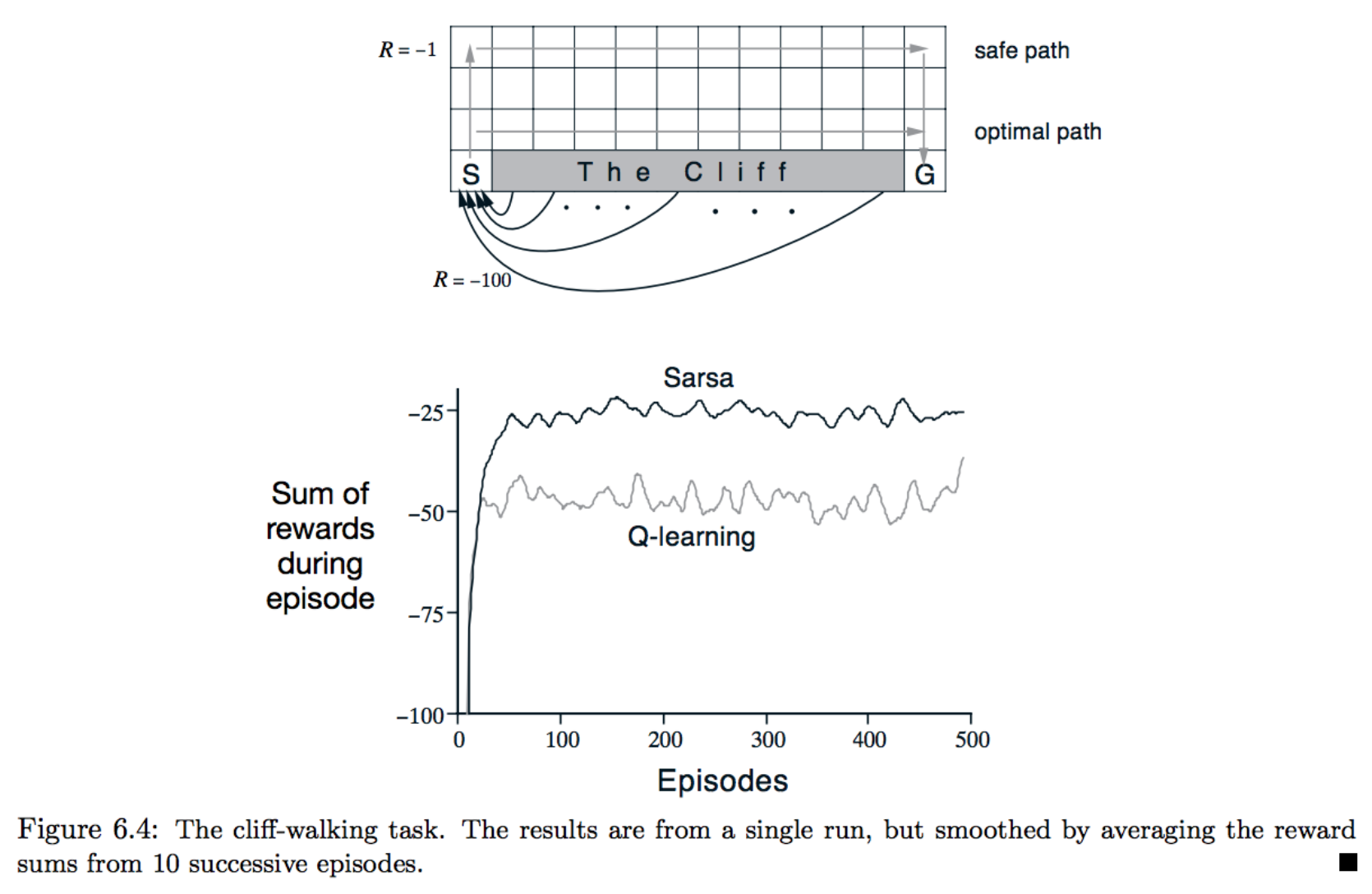
The figure shows the performance of Sarsa and Q-learning on the cliff walking environment for constant ϵ=0.1. As described in the textbook, in this case,

Q-learning achieves worse online performance (where the agent collects less reward on average in each episode), but learns the optimal policy, and Sarsa achieves better online performance, but learns a sub-optimal “safe” policy.

1-5-7 : Quiz: Check Your Understanding

you learned about many different algorithms for Temporal-Difference (TD) control. Later in this nanodegree, you’ll learn more about how to adapt the Q-Learning algorithm to produce the Deep Q-Learning algorithm that demonstrated superhuman performance at Atari games.

Before moving on, you’re encouraged to check your understanding by completing this brief quiz on Q-Learning.

from IPython.display import Image
Image(filename='./images/1-5-7-1_td_methods_quiz_agent_and_environment.png')

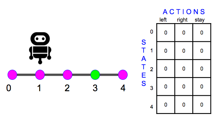
The Agent and Environment

Imagine an agent that moves along a line with only five discrete positions (0, 1, 2, 3, or 4). The agent can move left, right or stay put. (If the agent chooses to move left when at position 0 or right at position 4, the agent just remains in place.)

The Q-table has:

five rows, corresponding to the five possible states that may be observed, and three columns, corresponding to three possible actions that the agent can take in response. The goal state is position 3, but the agent doesn’t know that and is going to learn the best policy for getting to the goal via the Q-Learning algorithm (with learning rate α=0.2). The environment will provide a reward of -1 for all locations except the goal state. The episode ends when the goal is reached.

Episode 0, Time 0

The Q-table is initialized like below…

from IPython.display import Image
Image(filename='./images/1-5-7-2_td_methods_quiz_episode0_time0.png')

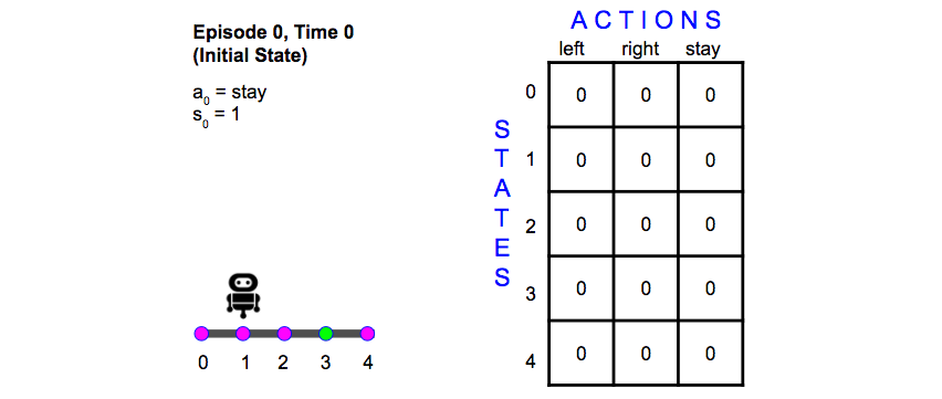
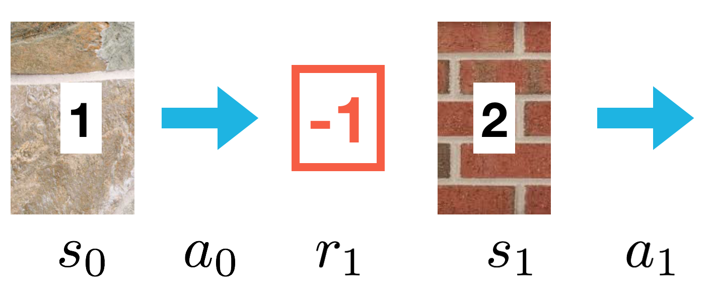
ay the agent observes the initial state (position 1) and selects action stay.

As a result, it receives the next state (position 1) and a reward (-1.0) from the environment.

Let:

• st denote the state at time step t,
• at denote the action at time step t, and
• rt denote the reward at time step t.

Then, the agent now knows s0,a0,r1 and s1. Namely, s0=1,a0=stay,r1=−1.0, and s1=1.

from IPython.display import Image
Image(filename='./images/1-5-7-3_td_methods_quiz_episode0_time0_q-table-update.png')

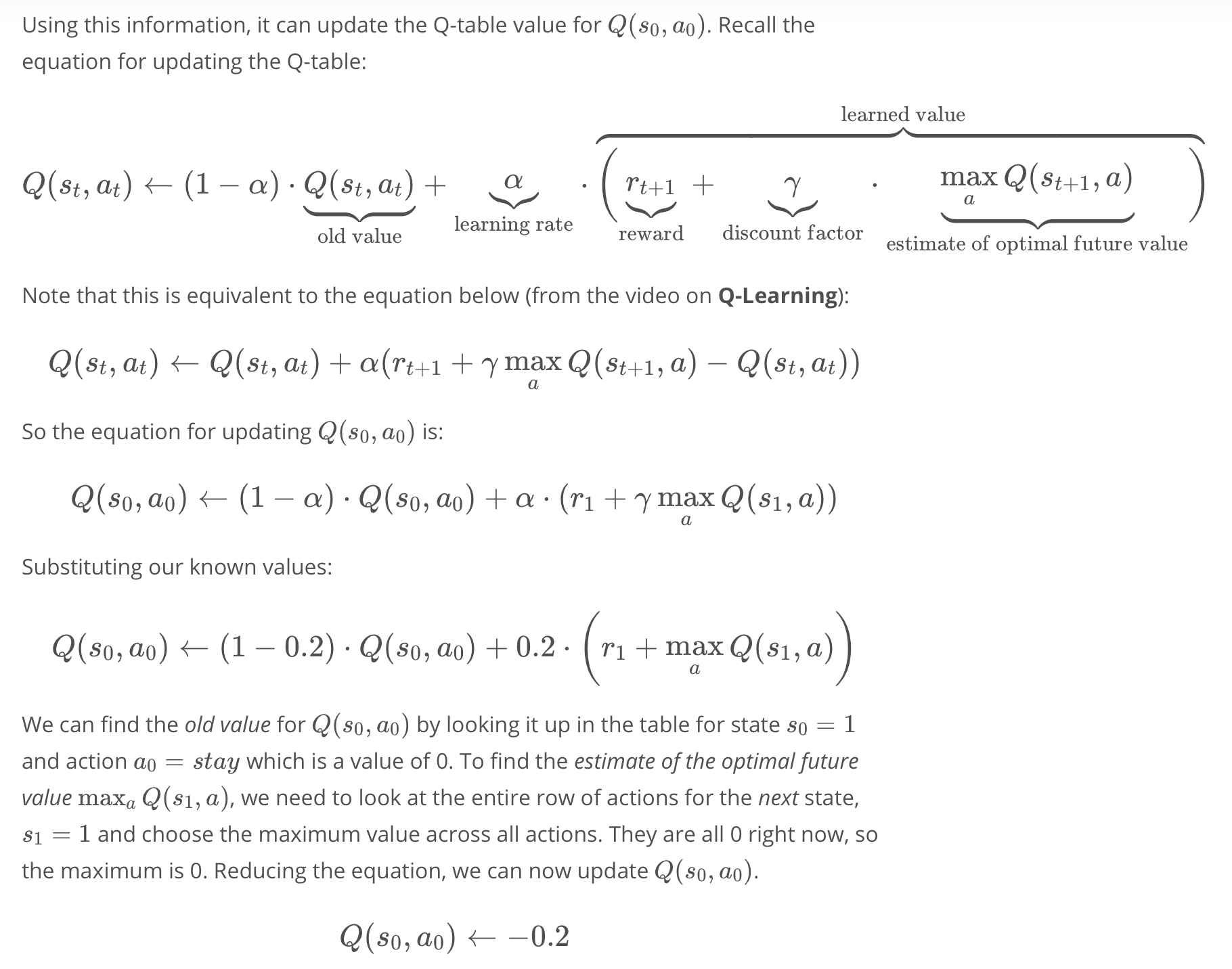
Episode 0, Time 1

from IPython.display import Image
Image(filename='./images/1-5-7-4_td_methods_quiz_episode0_time1.png')

At this step, an action must be chosen. The best action for position 1 could be either “left” or “right”, since their values in the Q-table are equal.

Remember that in Q-Learning, the agent uses the epsilon-greedy policy to select an action. Say that in this case, the agent selects action right at random.

Then, the agent receives a new state (position 2) and reward (-1.0) from the environment.

The agent now knows s1,a1,r2 and s2.

QUESTION 1 OF 2

What is the updated value for Q(s1,a1)? (round to the nearest 10th)

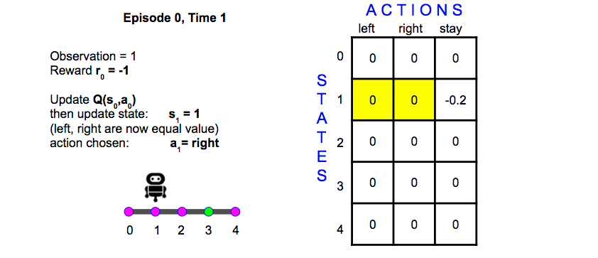
Episode n

Now assume that a number of episodes have been run, and the Q-table includes the values shown below.

A new episode begins, as before. The environment gives an initial state (position 1), and the agent selects action stay.

from IPython.display import Image
Image(filename='./images/1-5-7-5_td_methods_quiz_episode-n.png')

QUESTION 2 OF 2

What is the new value for Q(1,stay)? (round your answer to the nearest 10th)