RL in Continuous Spaces

from IPython.display import Image
Image(filename='./images/1-0-0-1_opening.jpg')

Lesson 1-6: RL in Continuous Spaces

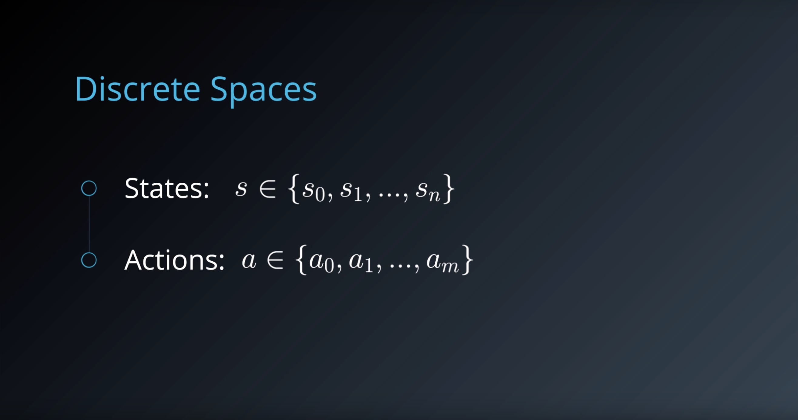
So far, you have worked with reinforcement learning environments where the number of states and actions is limited. With small, finite Markov Decision Processes (MDPs), it is possible to represent the action-value function with a table, dictionary, or other finite structure.

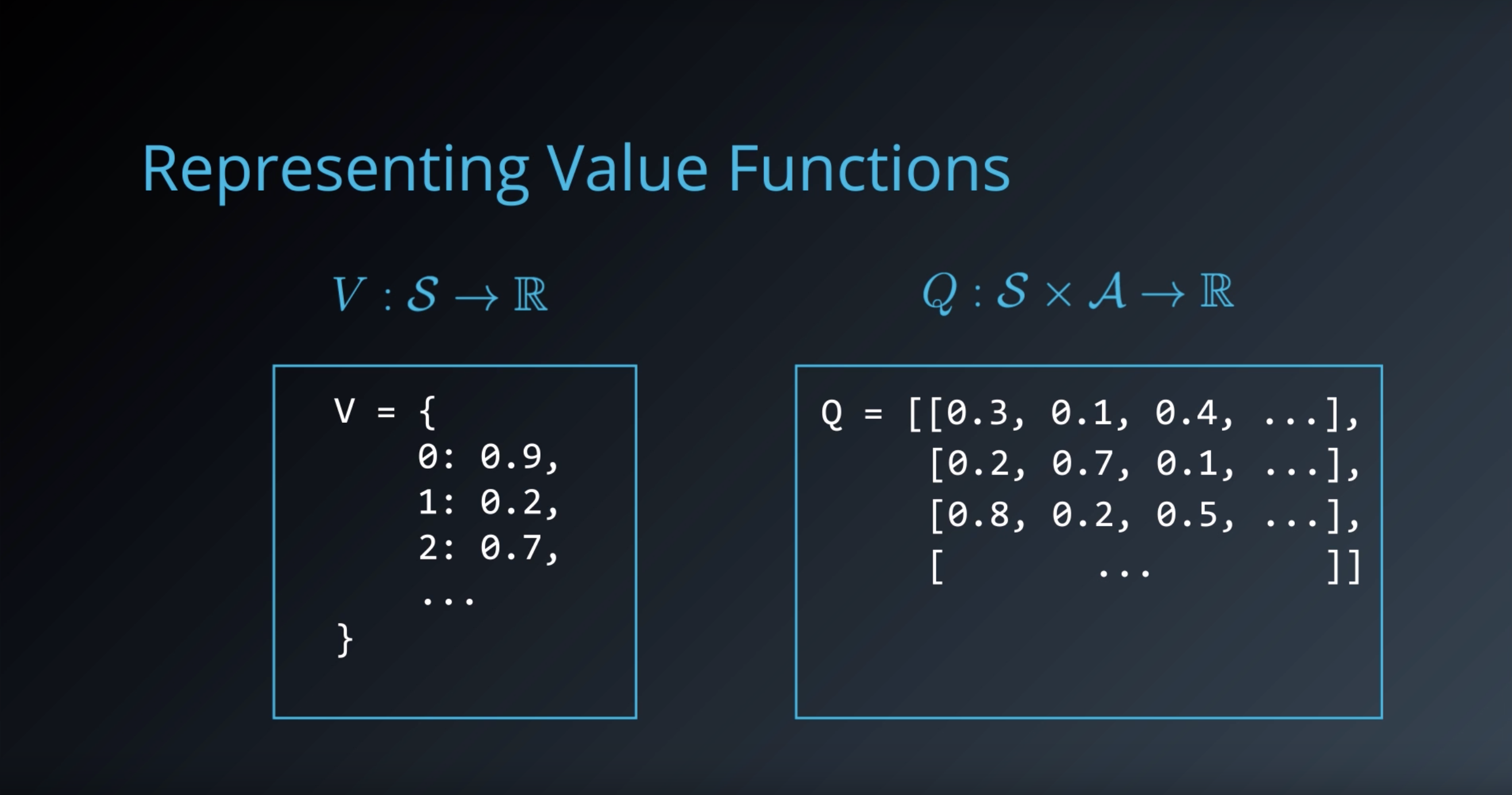
For instance, consider the very small gridworld below. Say the world has four possible states, and the agent has four possible actions at its disposal (up, down, left, right). You learned in the previous lessons that we can represent the estimated optimal action-value function in a table, with a row for each state and a column for each action. We refer to this table as a Q-table.

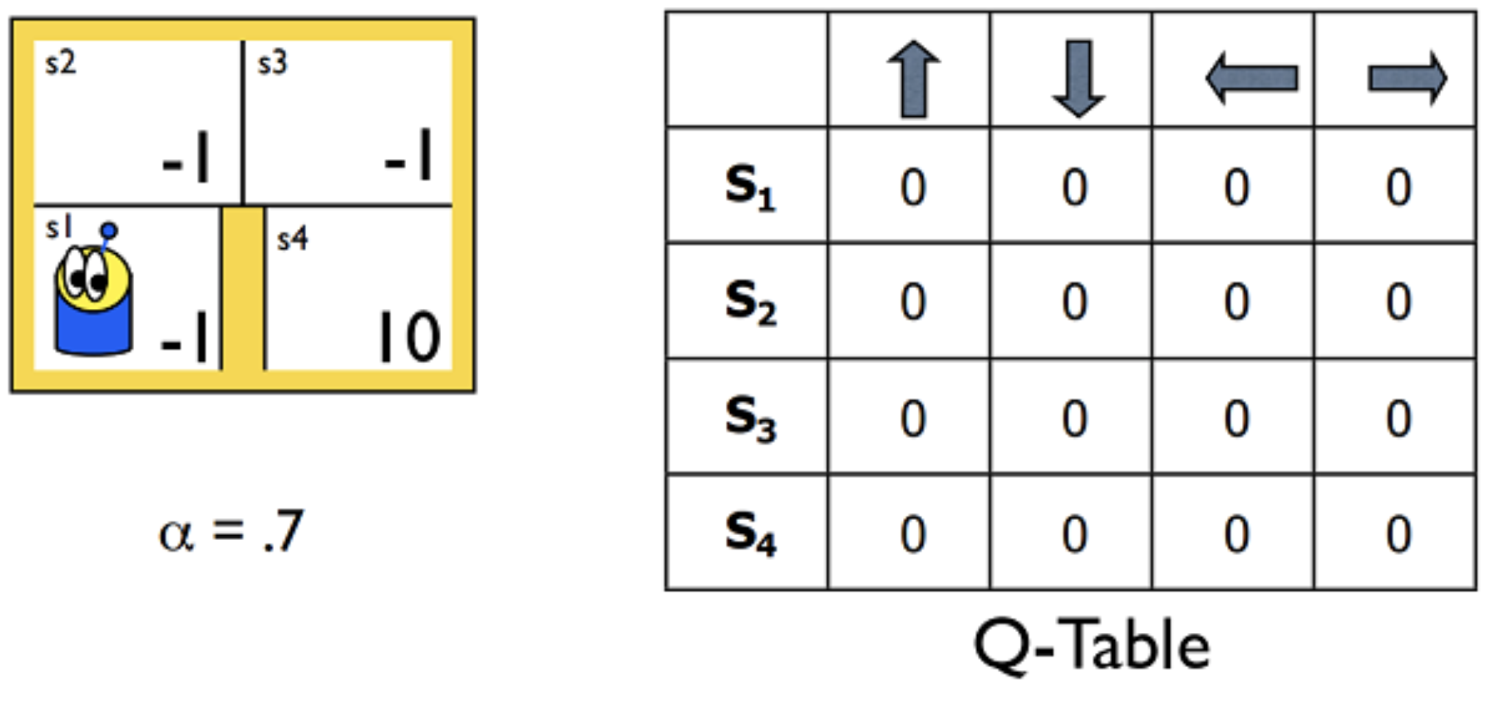
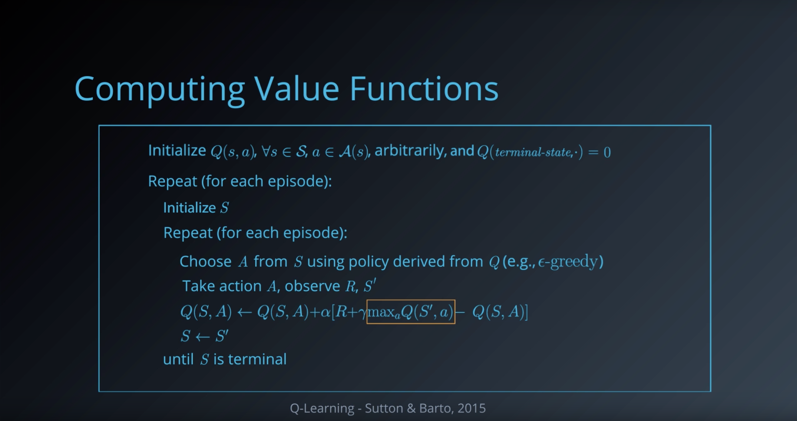
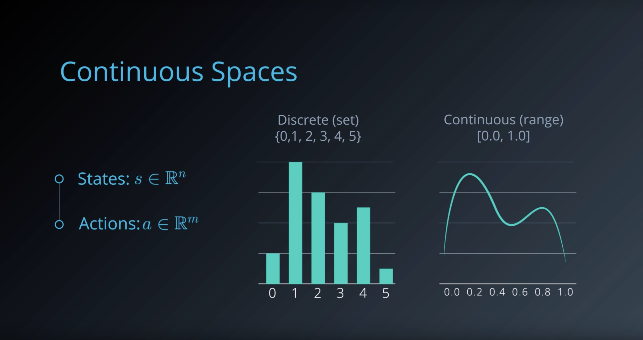
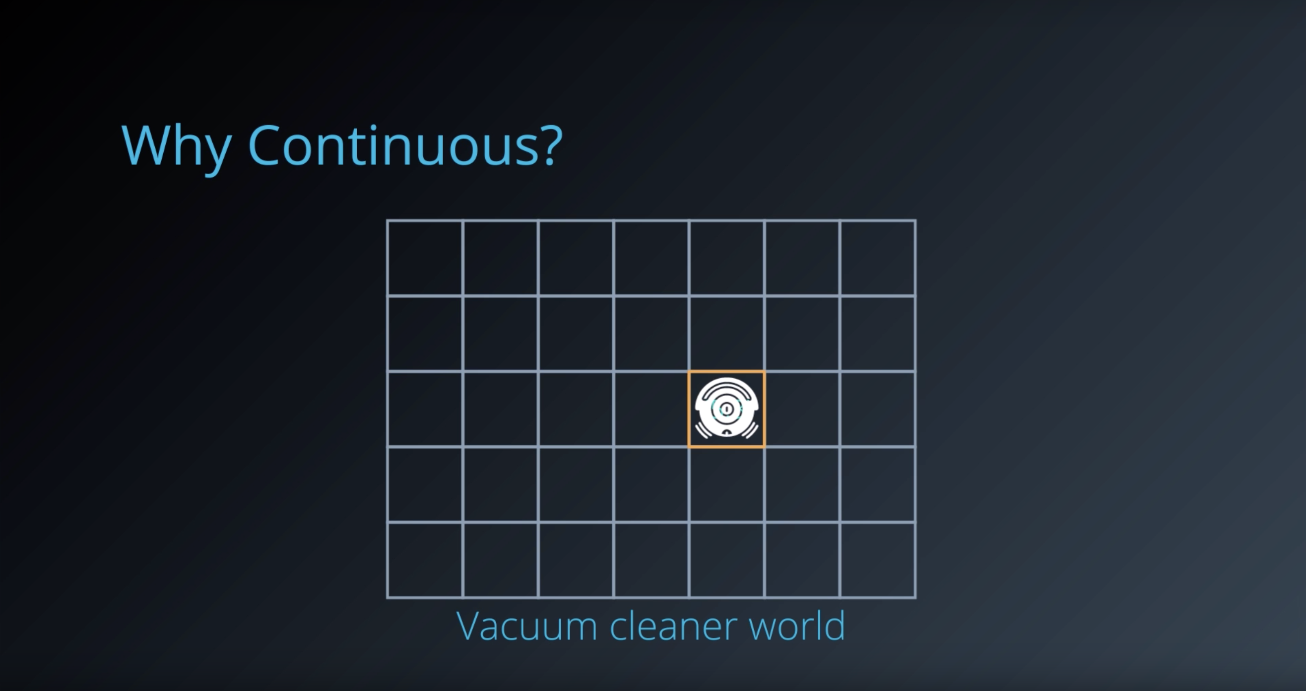
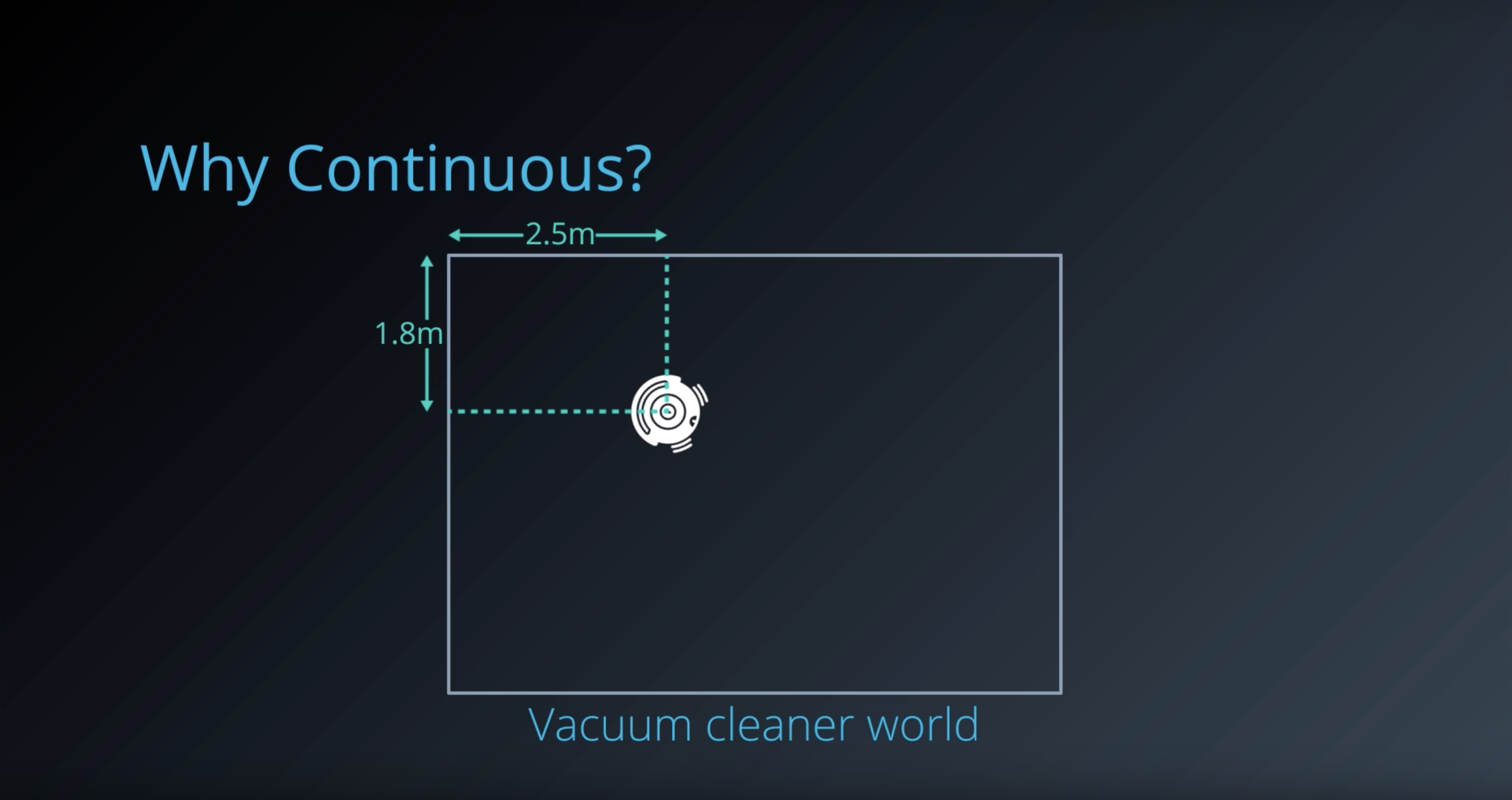
But what about MDPs with much larger spaces? Consider that the Q-table must have a row for each state. So, for instance, if there are 10 million possible states, the Q-table must have 10 million rows. Furthermore, if the state space is the set of continuous real-valued numbers (an infinite set!), it becomes impossible to represent the action values in a finite structure!

In this lecture, you will learn how to generalize the tabular solution methods from the previous lessons to work with large and continuous spaces. This will lay the foundation for developing the deep reinforcement learning algorithms that you will explore later in the nanodegree.

1-6-1 : Overview of RL framework

from IPython.display import Image
Image(filename='./images/1-6-1-1_overview_rl_mdp_and_policy.png')

from IPython.display import Image
Image(filename='./images/1-6-1-2_model-based-learning_and_model-free-learning.png')

from IPython.display import Image
Image(filename='./images/1-6-1-3_rl-in-continuous-learning_is_a_base_of_drl-algorithms.png')

1-6-2 : Discrete vs. Continuous Spaces

from IPython.display import Image
Image(filename='./images/1-6-2-1_discrete-space.png')

from IPython.display import Image
Image(filename='./images/1-6-2-2_representing_value-functions.png')

from IPython.display import Image
Image(filename='./images/1-6-2-3_computing_value-functions_value-interation.png')

from IPython.display import Image
Image(filename='./images/1-6-2-4_computing_value-functions_q-learning.png')

from IPython.display import Image
Image(filename='./images/1-6-2-5_continuous-spaces.png')

from IPython.display import Image
Image(filename='./images/1-6-2-6_why_continuous_descrete_example_is_easy_to_understand.png')

from IPython.display import Image
Image(filename='./images/1-6-2-7_why_continuous_but_real_world_is_continuous.png')

from IPython.display import Image
Image(filename='./images/1-6-2-8_continuous-actions.png')

from IPython.display import Image
Image(filename='./images/1-6-2-9_dealing_with_continuous-spaces.png')

Quiz

Which of the following state or action spaces can be encoded using discrete representations?

1. A hand of cards when playing Poker
2. Force applied when grasping with a robotic arm
3. GPS coordinates for autonomous driving
4. Board positions for a 9x9 Go game
5. Keys to play on a musical keyboard

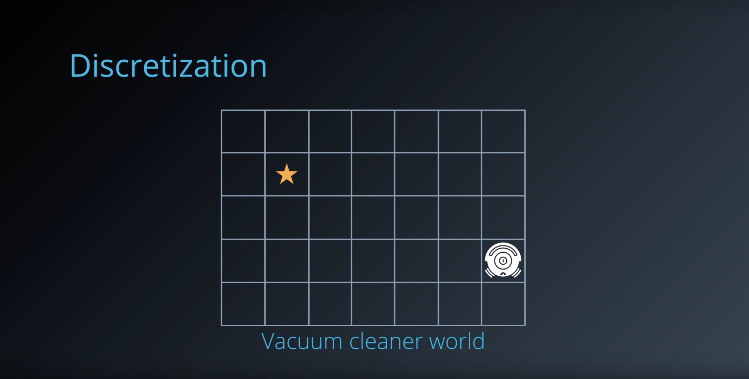
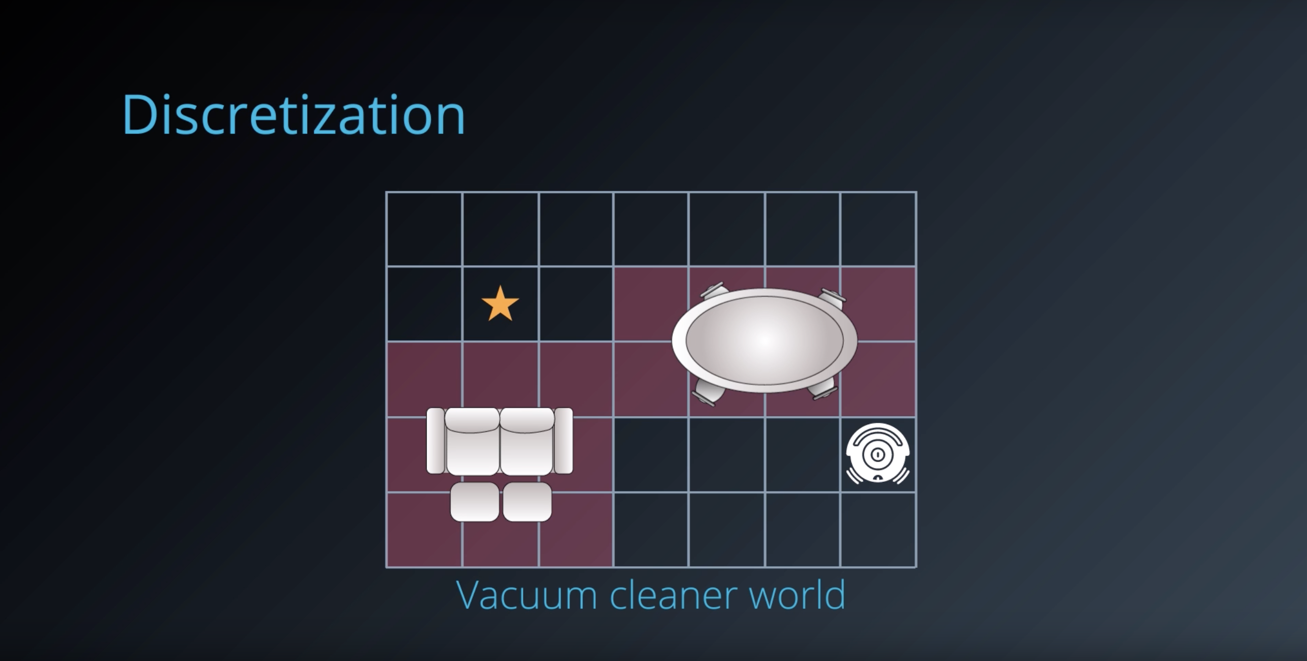
1-6-3. Discretization

from IPython.display import Image
Image(filename='./images/1-6-3-1_discertization_vacuum-clearner-world.png')

from IPython.display import Image
Image(filename='./images/1-6-3-2_discertization_vacuum-clearner-world_obstacle_with_no_path.png')

from IPython.display import Image
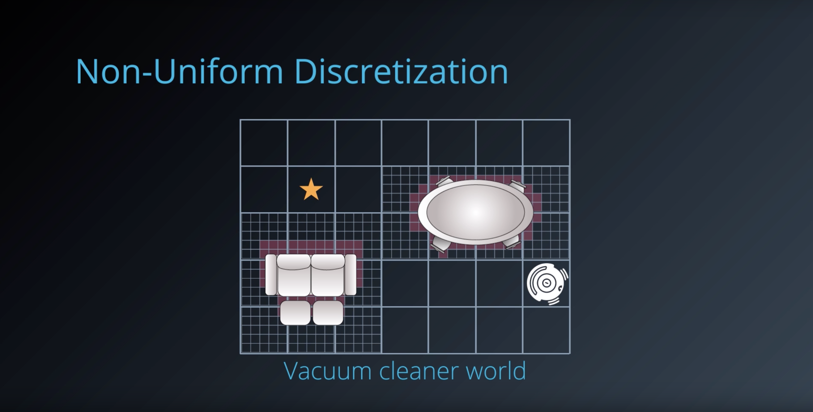
Image(filename='./images/1-6-3-3_discertization_vacuum-clearner-world_non-uniform-descretization_example_1.png')

from IPython.display import Image
Image(filename='./images/1-6-3-4_discertization_vacuum-clearner-world_non-uniform-descretization_example_2.png')

from IPython.display import Image
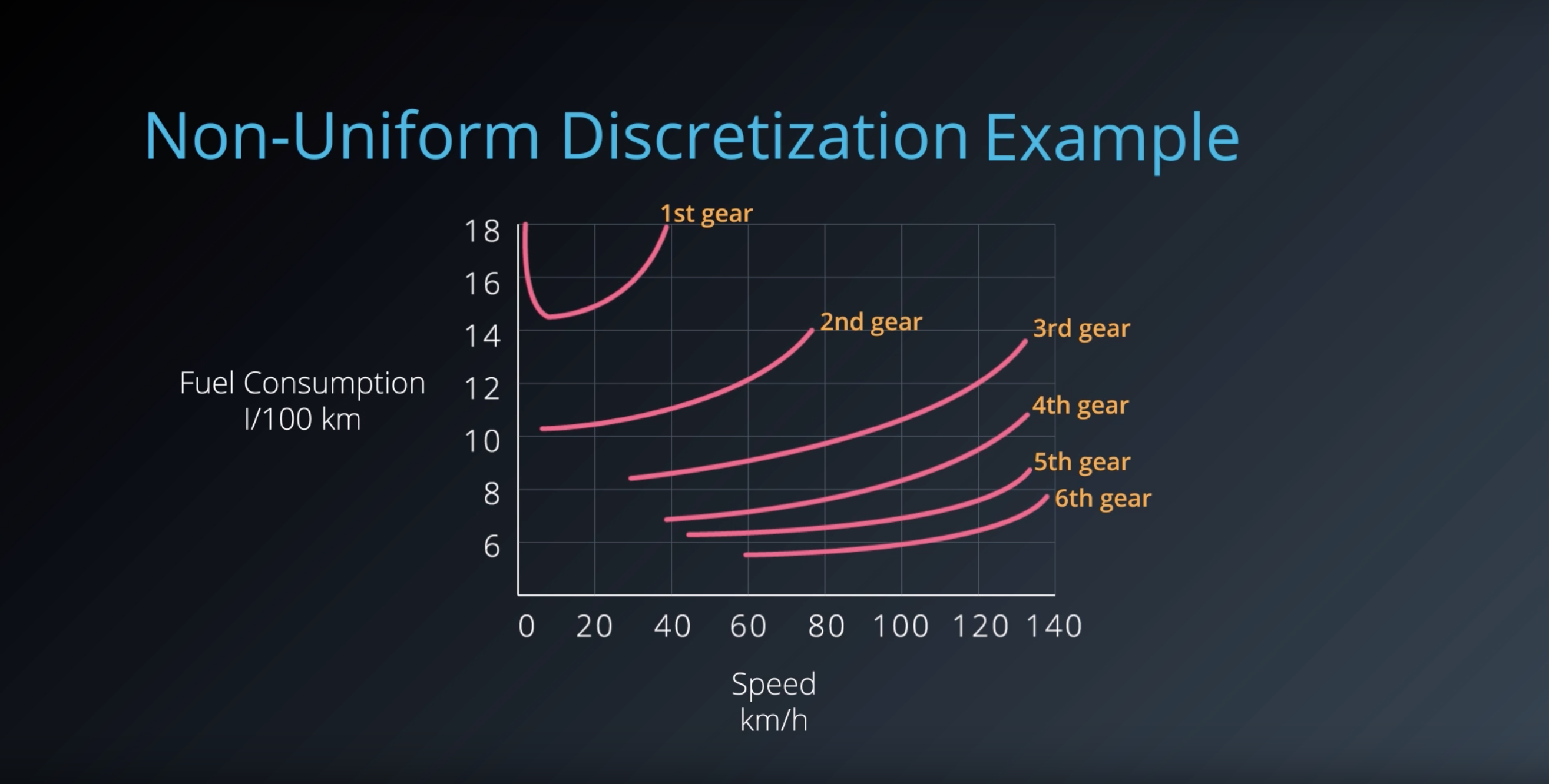
Image(filename='./images/1-6-3-5_discertization_other_non-uniform-descretization_example.png')

from IPython.display import Image
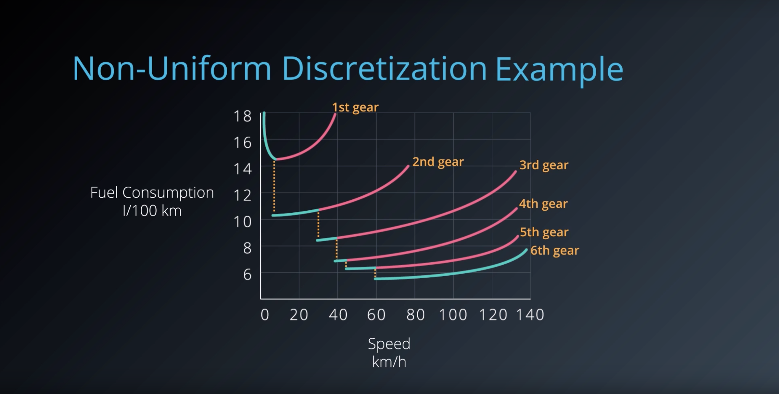
Image(filename='./images/1-6-3-6_discertization_other_non-uniform-descretization_example.png')

1-6-4 : Tile Coding

from IPython.display import Image
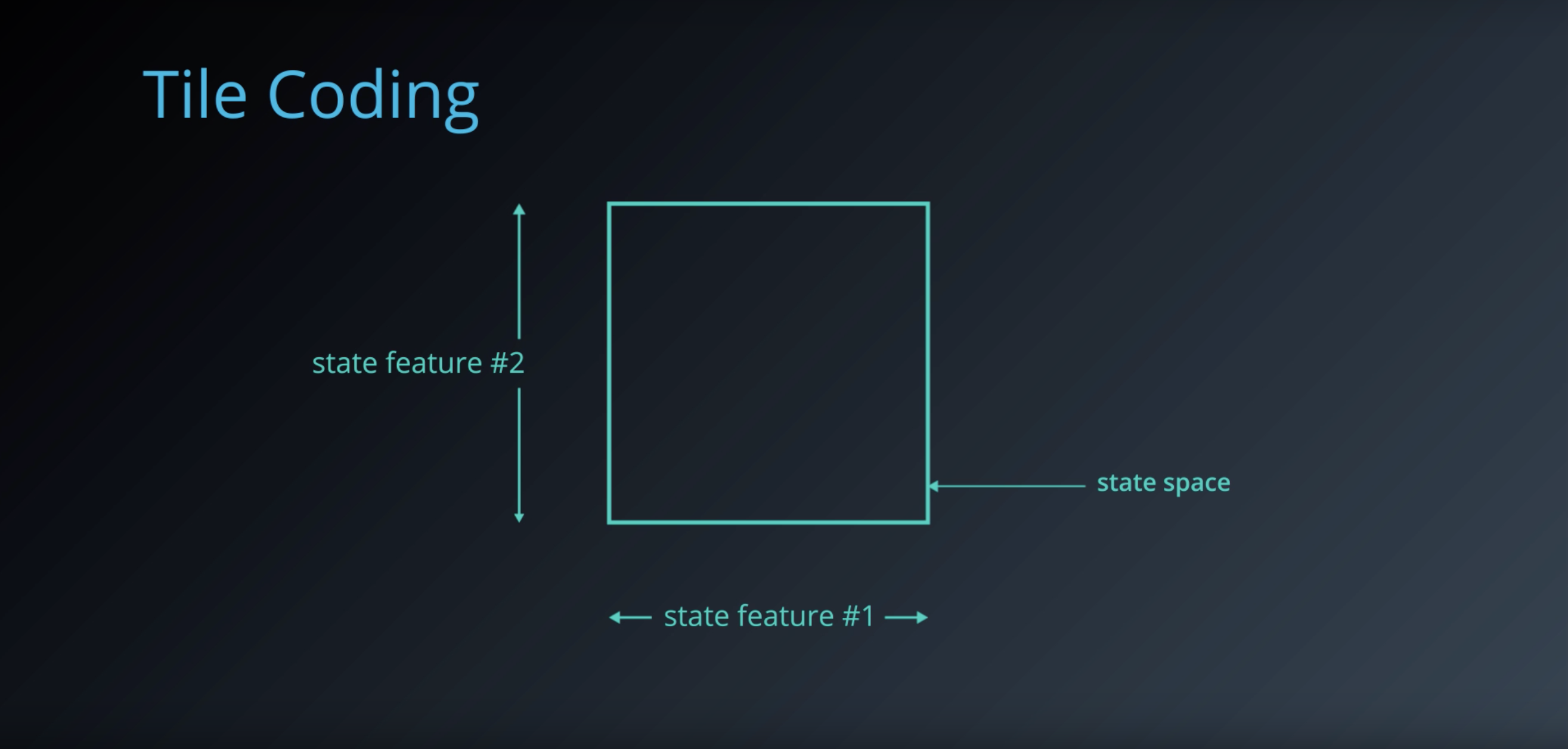
Image(filename='./images/1-6-4-1_tile-coding_state_space_is_continous_and_two_dimentional.png')

from IPython.display import Image
Image(filename='./images/1-6-4-2_tile-coding_overlay_multiple_tilings_on_top_of_the_space.png')

from IPython.display import Image
Image(filename='./images/1-6-4-3_tile-coding_each_slightly_offset_from_each_other.png')

from IPython.display import Image
Image(filename='./images/1-6-4-4_tile-coding_position_s_is_coarsly_identified_by_the_tiles.png')

from IPython.display import Image
Image(filename='./images/1-6-4-5_tile-coding_it_represent_new_discretised_state_as_a_bit_vector.png')

from IPython.display import Image
Image(filename='./images/1-6-4-6_tile-coding_algorithm.png')

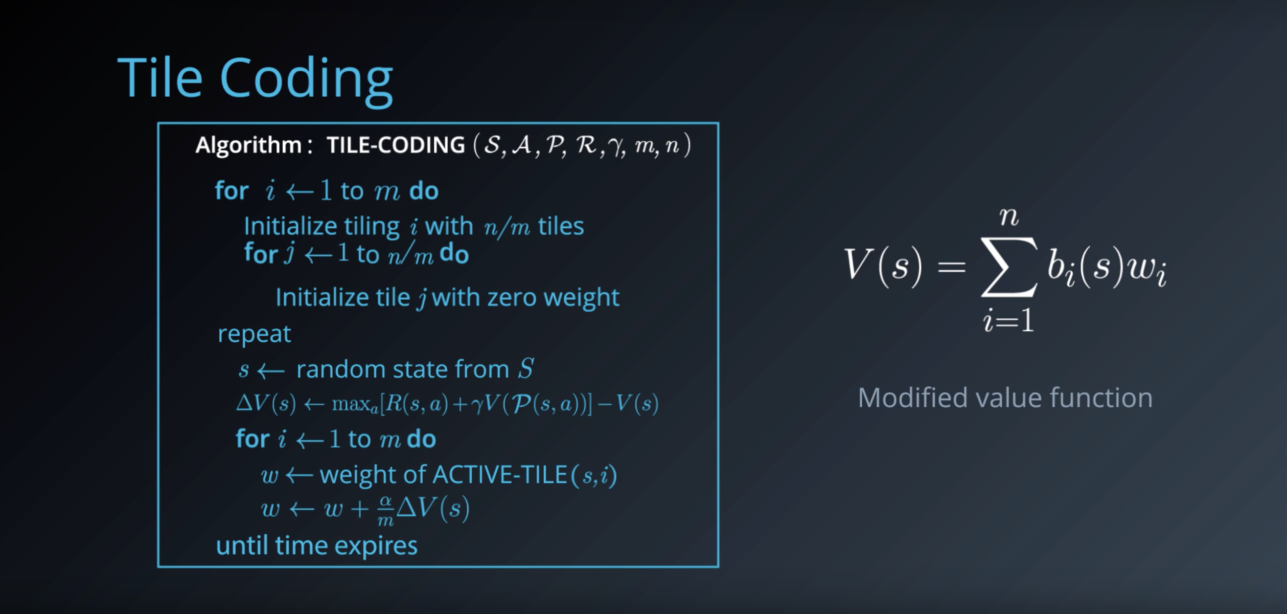
The point is how the state value fuction is computed.

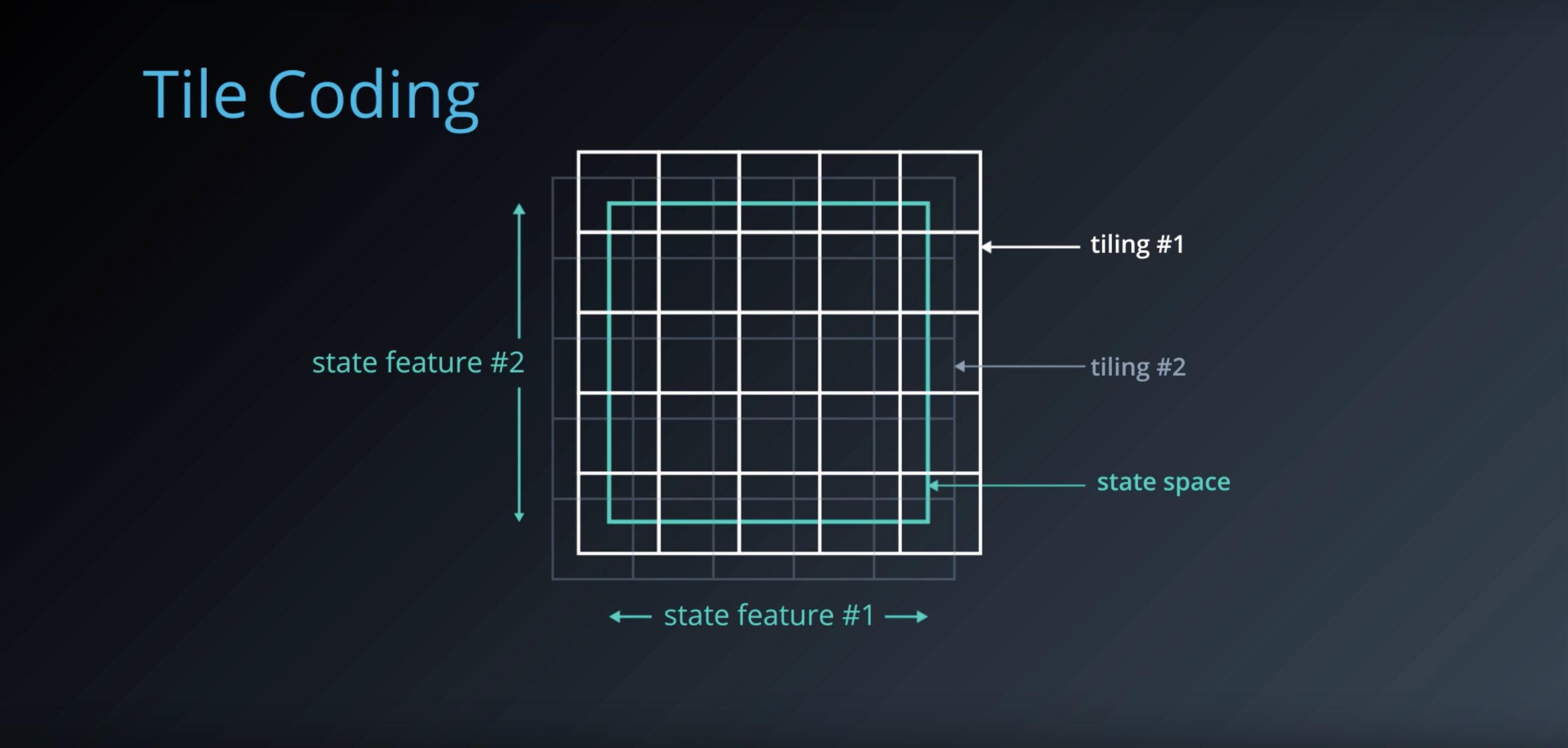
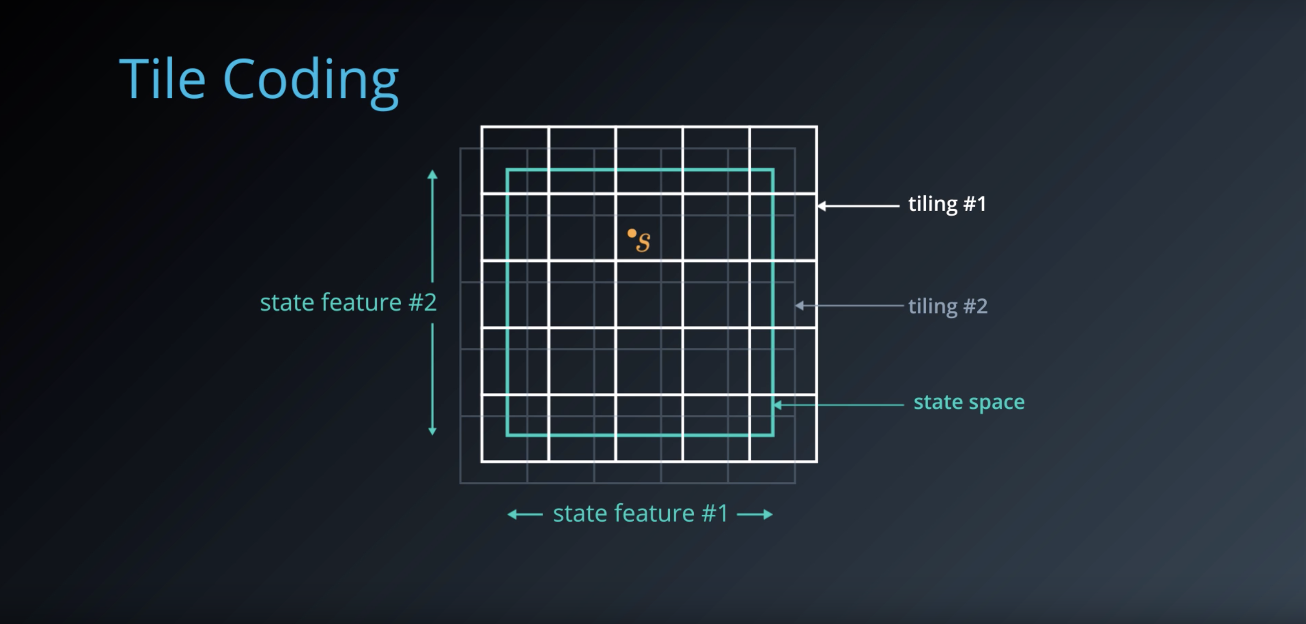
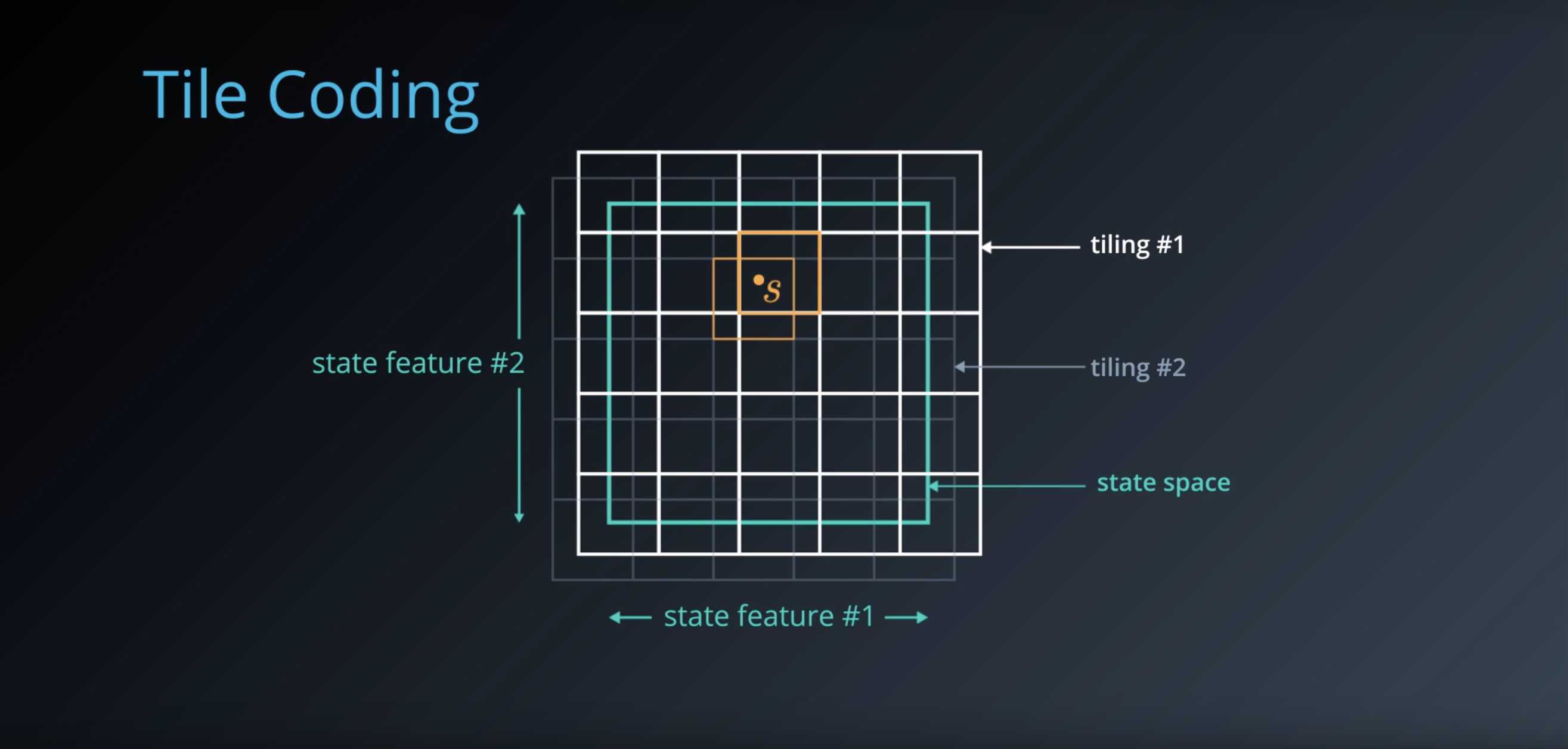
• Instead of storing a separate value for each stave V of S, it is defined in terms of the bit vector for that state and a weight for each tile.
• The tile coding algorithm in turn updates these weights iteratively.
• This ensures nearby loactions that share tiles also share state value.

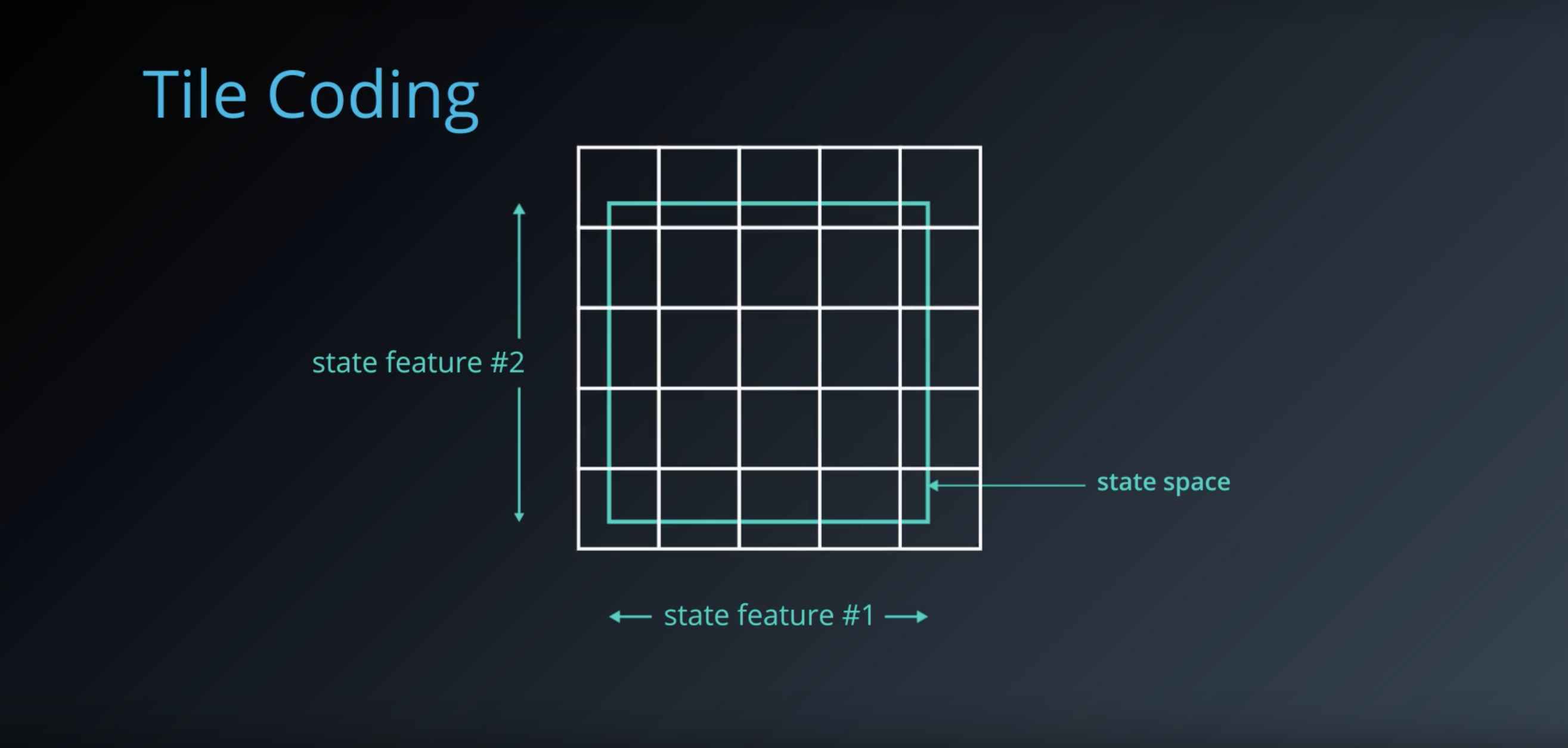
Tile coding does have some drawbacks. we have to manually select the tile sizes,

from IPython.display import Image
Image(filename='./images/1-6-4-7_adaptive-tile-coding.png')

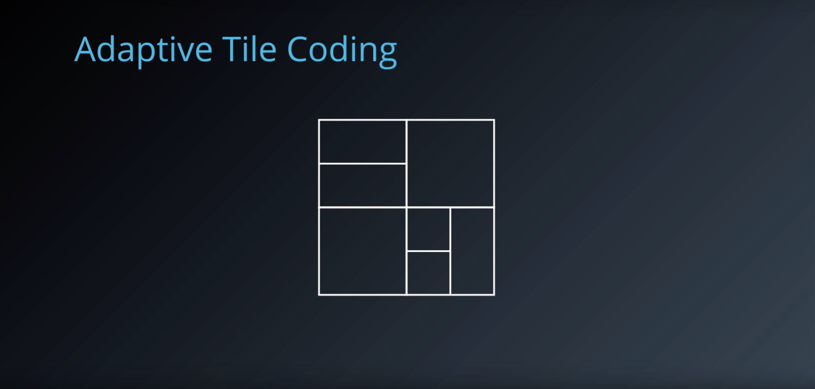
Adaptive Tile Coding is more flexibile approach.

• It start with fairly large tiles and divides each tile into two whenever appropriate.
• Basically, we want to split the state space when we realize that we are no longer learning much with currunt representation. This is, when our value function isn’t changing or some max iterations.
• In order to figure out which tile to split, we have to look at which one is likely to have the greatest effect on the value function. For this, we need to keep track of subtiles and their projected weights. Then, we can pick the title with the greatest difference between subtile weights.

The main advantage is that it doesn’t rely on a human to specify a discretisation ahead of time.

The resulting state space is appropriately partitioned based on its complexity.

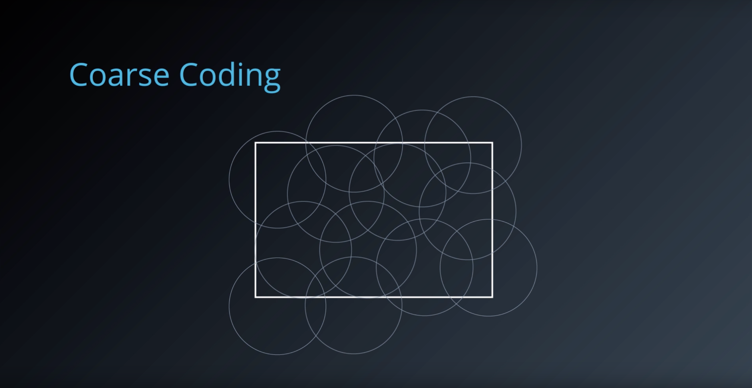
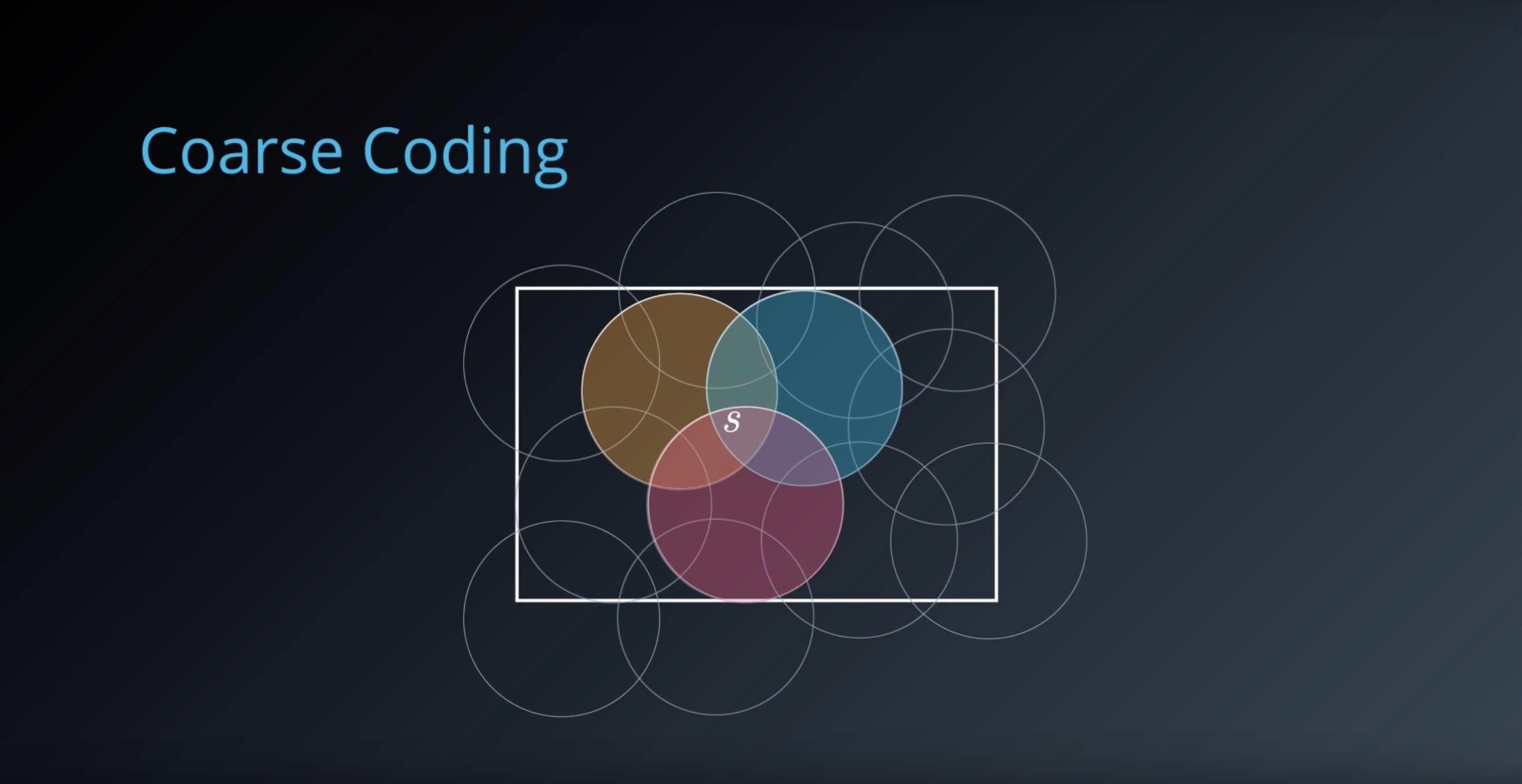
1-6-5 : Coarse Coding

from IPython.display import Image
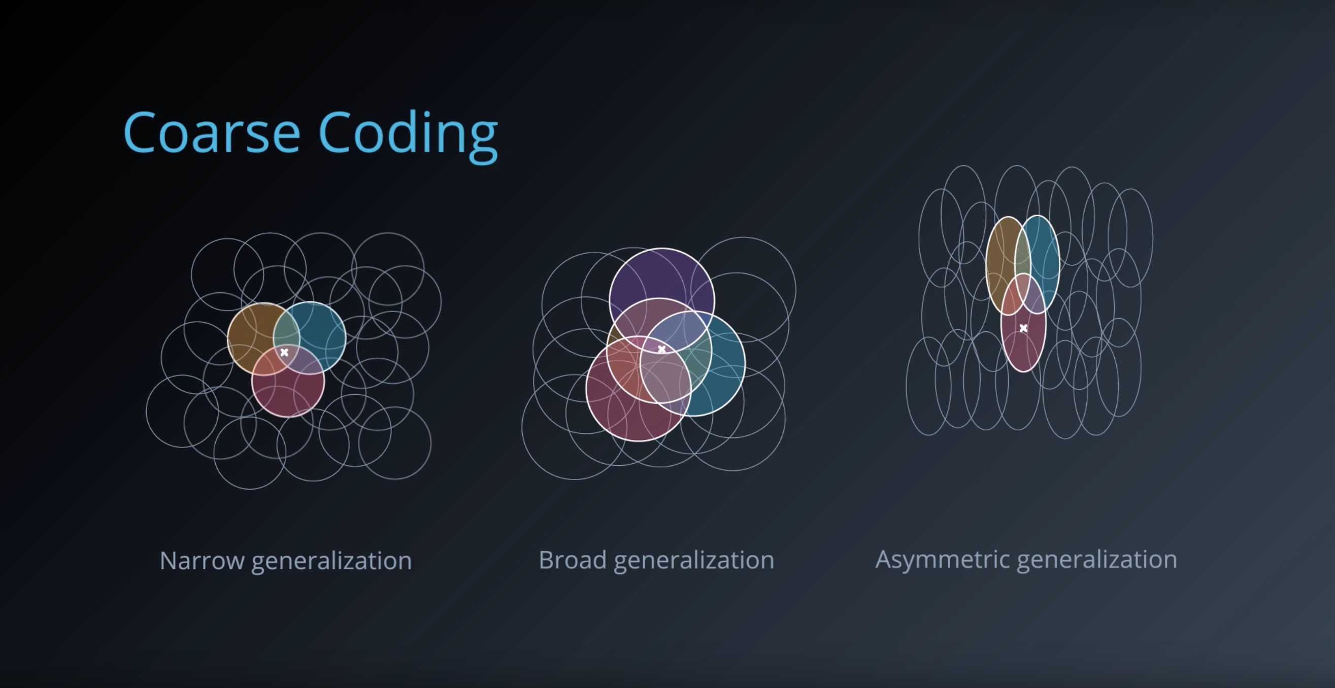
Image(filename='./images/1-6-5-1_course-coding_uses_a_sparser_set_of_features_to_encode_state_space.png')

from IPython.display import Image
Image(filename='./images/1-6-5-2_course-coding_prepare_a_bit_vector_with_1_for_those_circles_and_0_for_the_rest.png')

from IPython.display import Image
Image(filename='./images/1-6-5-3_course-coding_three_generalizations.png')

from IPython.display import Image
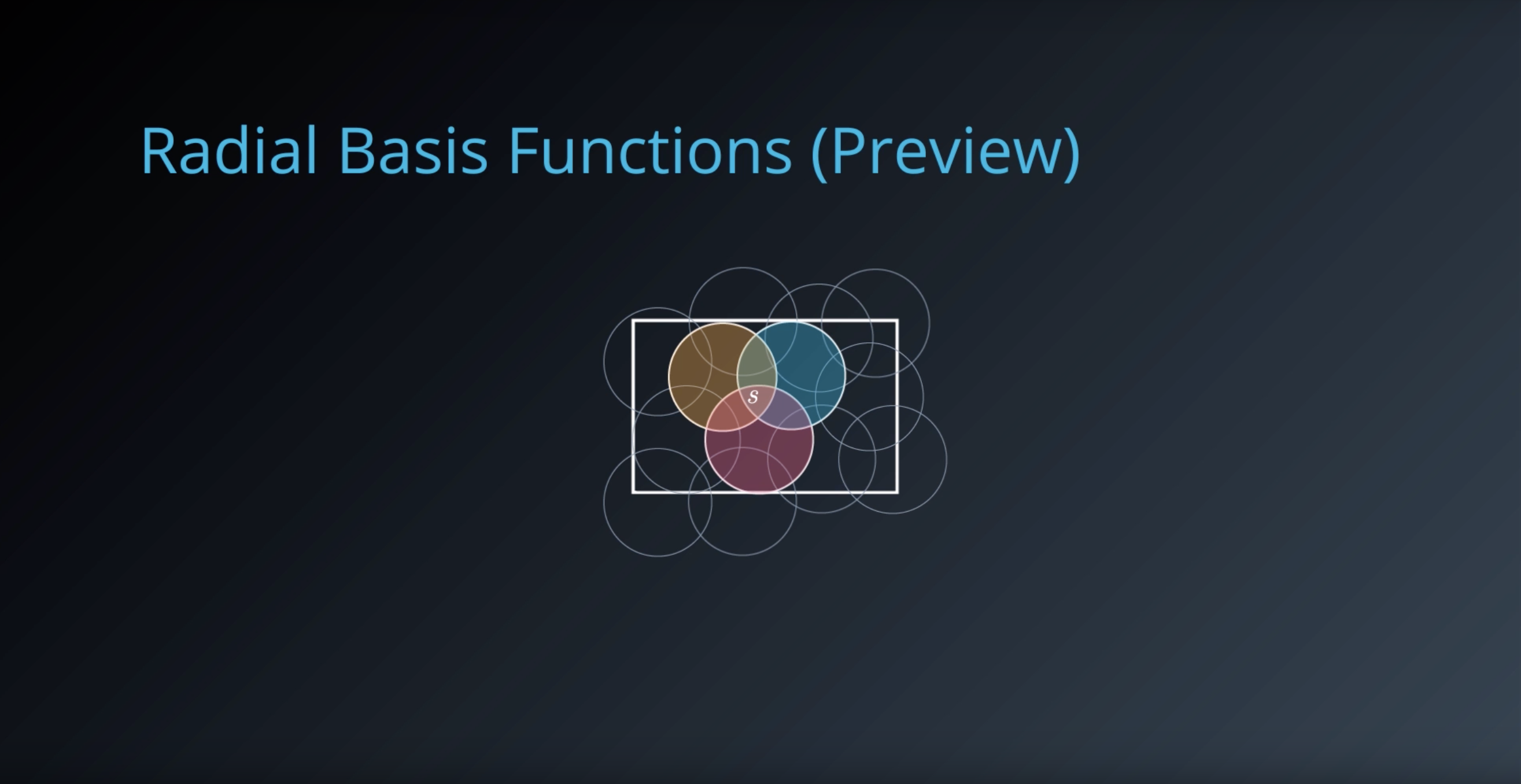
Image(filename='./images/1-6-5-4_course-coding_RadialBasisFunctions.png')

from IPython.display import Image
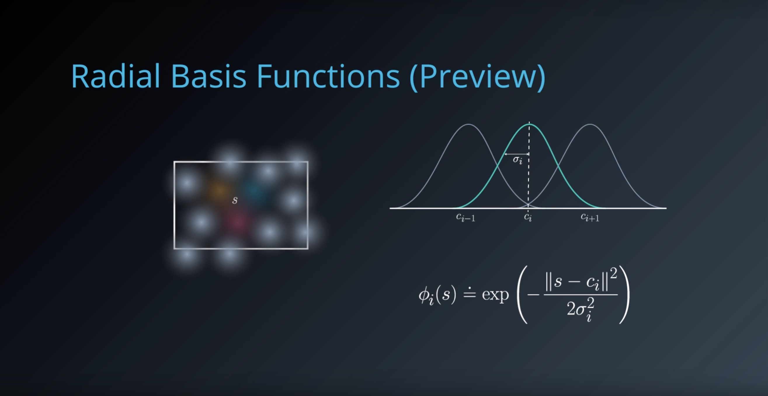
Image(filename='./images/1-6-5-5_course-coding_RadialBasisFunctions_is_cool_that_the_number_of_features_can_be_drastically_reduced.png')

1-6-6 : Function Approximation

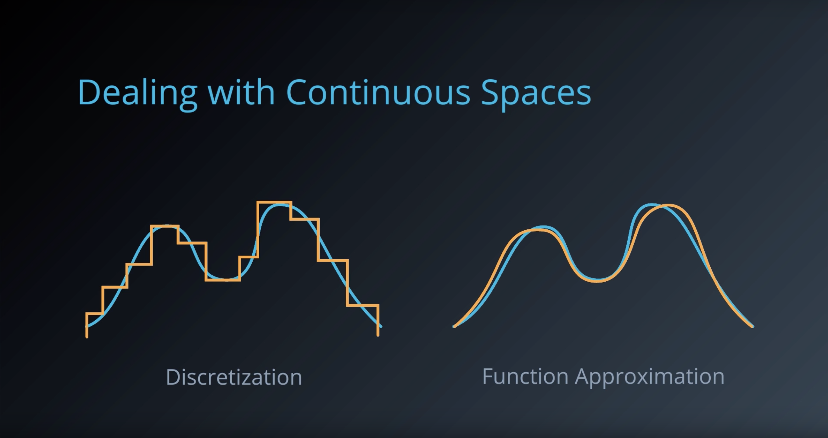
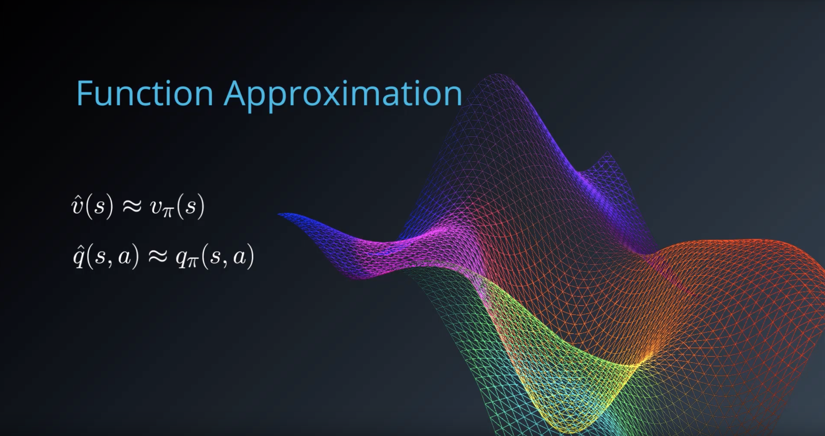
So far, we’ve looked at ways to discretize continous state spaces. This enables us to use existing traditional reinforcement learning algorithms with little or no modification.

But there are some limitations.

• When the underlying space is complicated, the number of discrete states needed can become vary very large.
• We lose the advantage of discretization.
• Moreover, if you think about positions in the state space that are nearby, you would expect their values to be similar, or smoothly changing.

Discertization doesn’t always exploit this characteristic, failing to generalize well across the space.

from IPython.display import Image
Image(filename='./images/1-6-6-1_fa_capturing_ture_state_value_completely_is_practically_infeasible.png')

from IPython.display import Image
Image(filename='./images/1-6-6-2_fa_approximation_is_best_hope_because_we_dont_know_what_the_function_is.png')

from IPython.display import Image
Image(filename='./images/1-6-6-3_fa_our_task_is_tweaking_this_parameter_vector_till_we_find_the_desired_approximation.png')

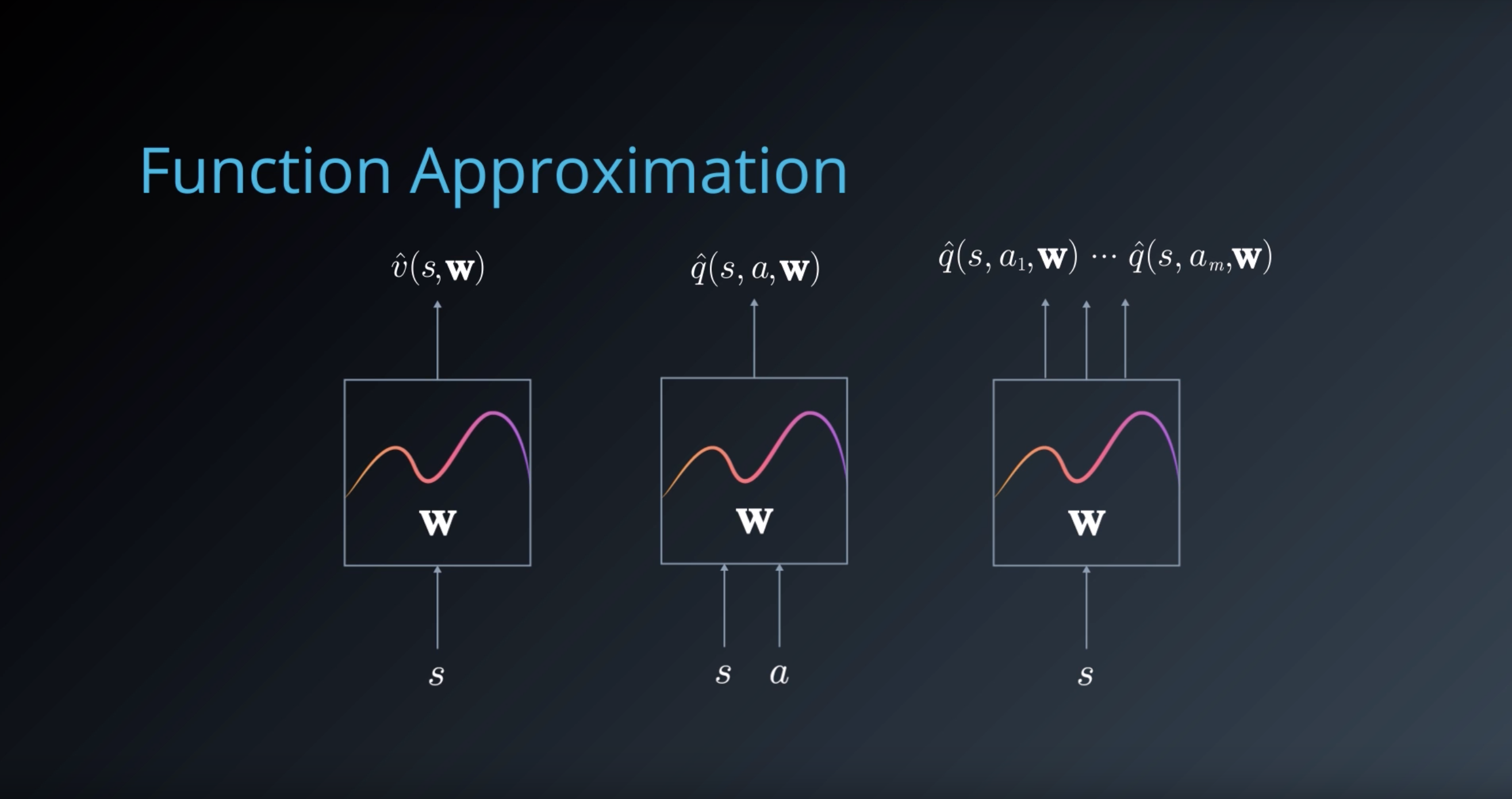
from IPython.display import Image
Image(filename='./images/1-6-6-4_fa_magic_is_converting_the_state_s_into_scalar_value.png')

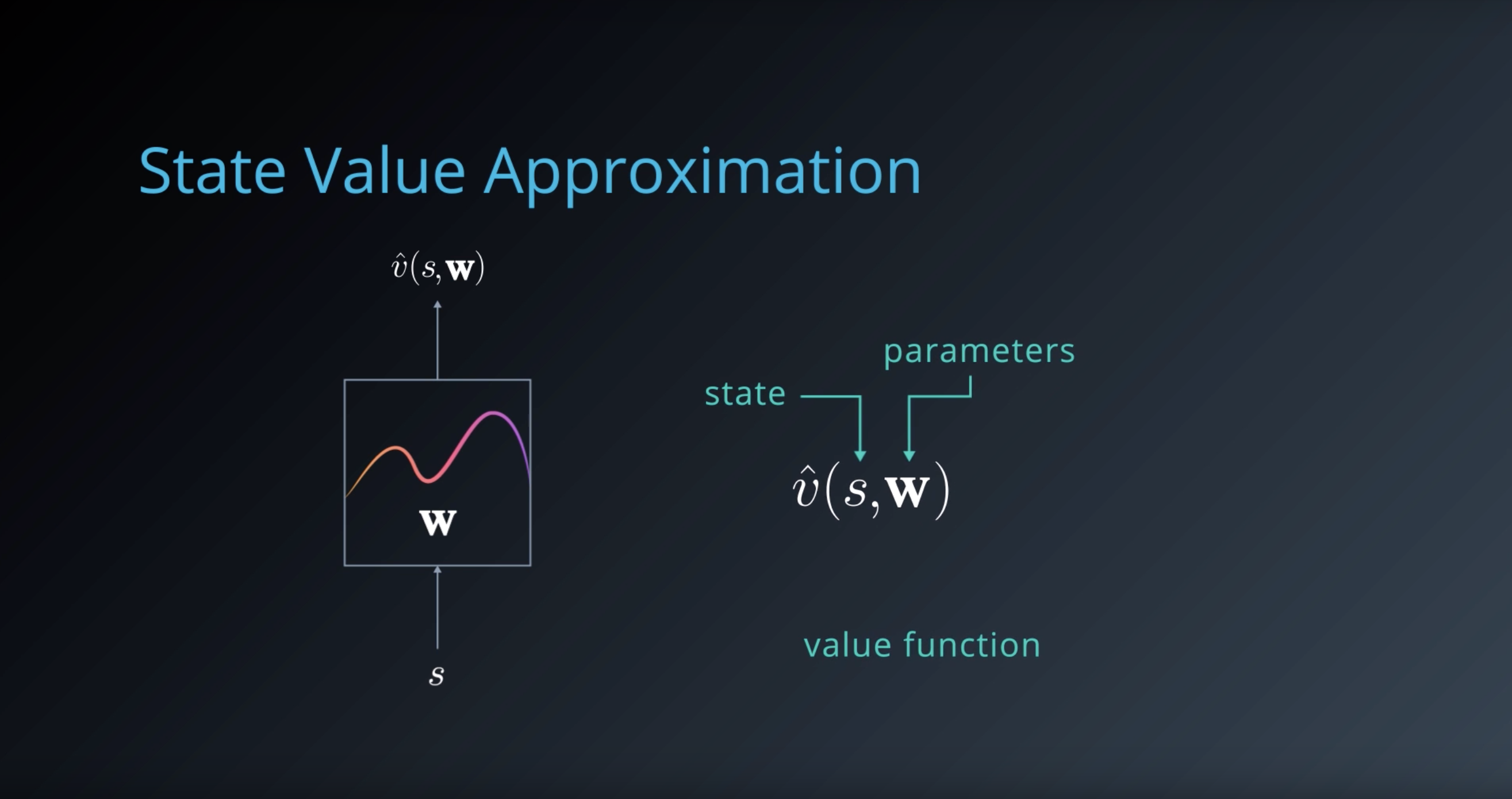
from IPython.display import Image
Image(filename='./images/1-6-6-5_fa_the_first_thing_is_to_ensure_feature_vector_that_represents_the_state.png')

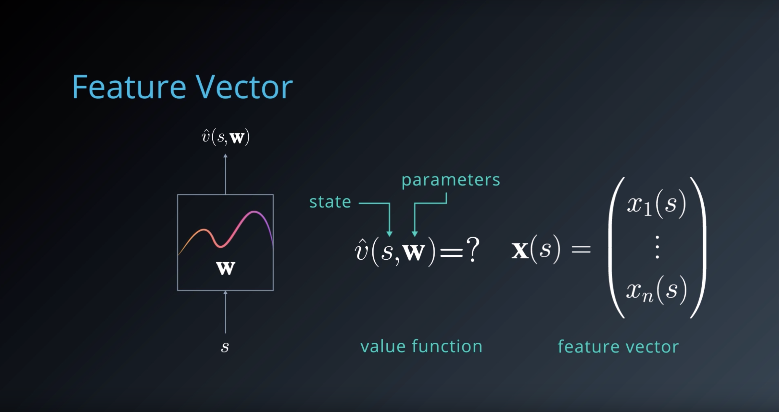
from IPython.display import Image
Image(filename='./images/1-6-6-6_fa_this_is_the_same_as_computing_a_linear_combination_of_features.png')

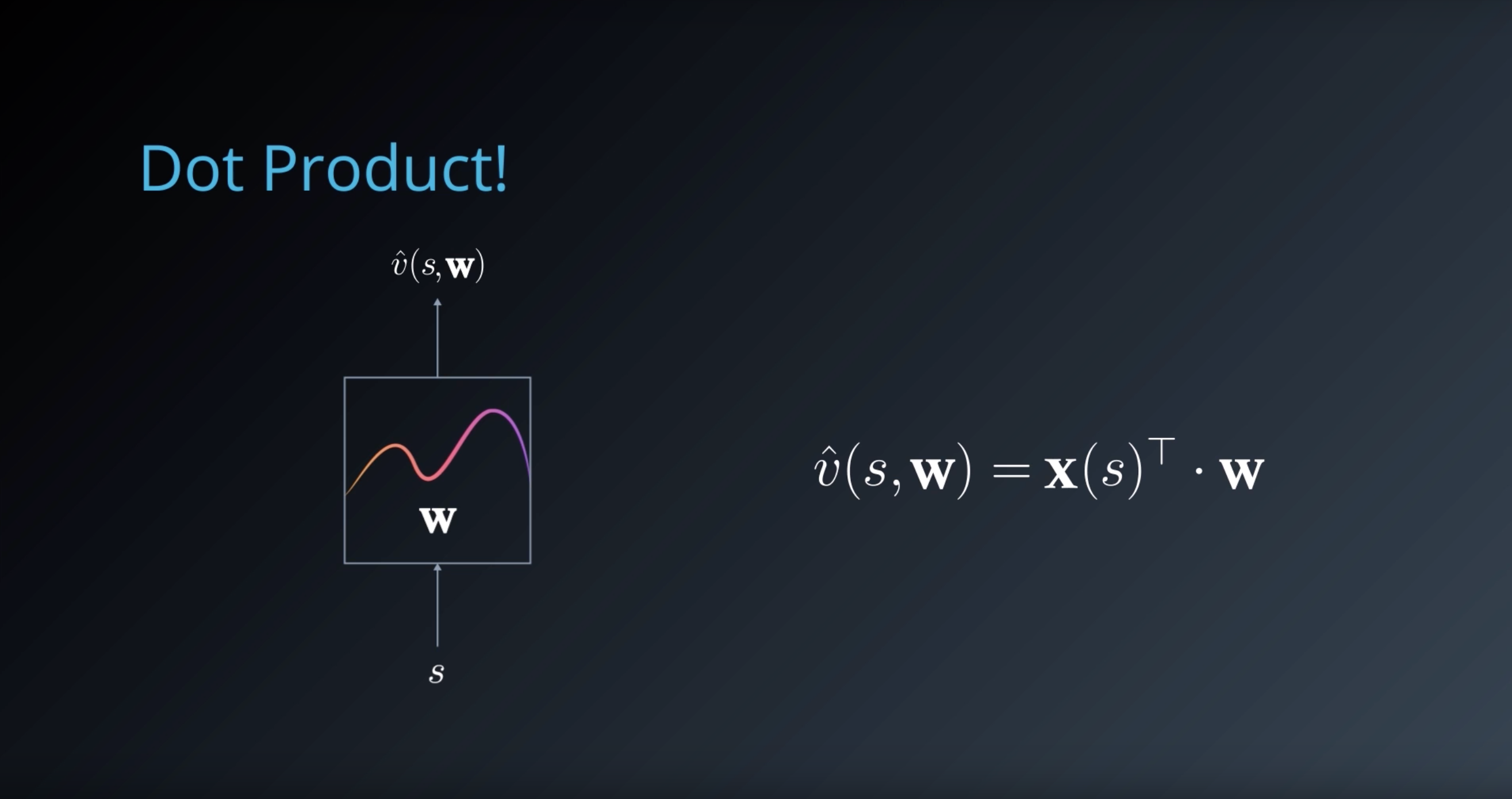
from IPython.display import Image
Image(filename='./images/1-6-6-7_fa_multiplying_each_feature_with_the_corresponding_weight_and_sum_it_up.png')

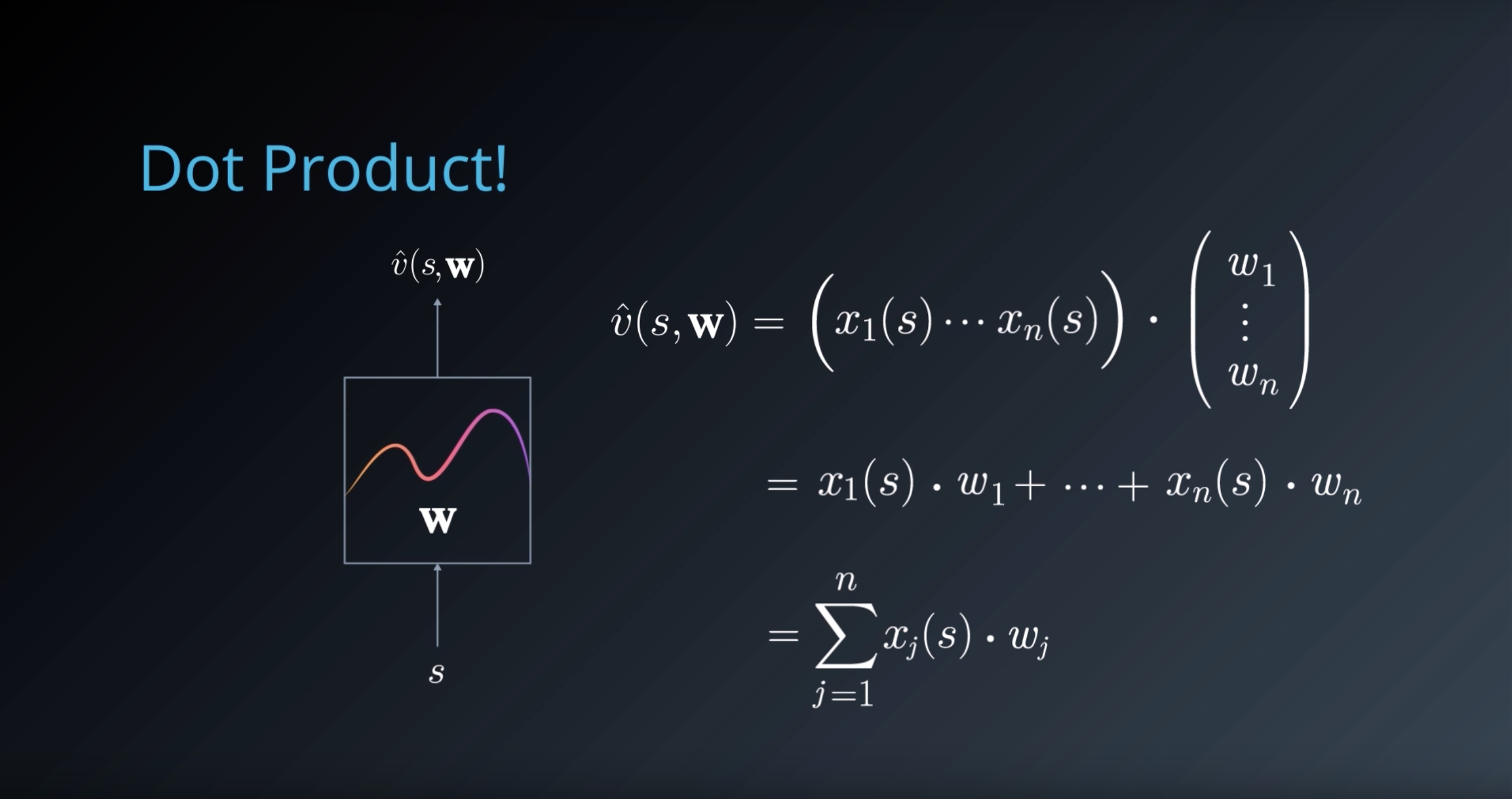
Function Approximation

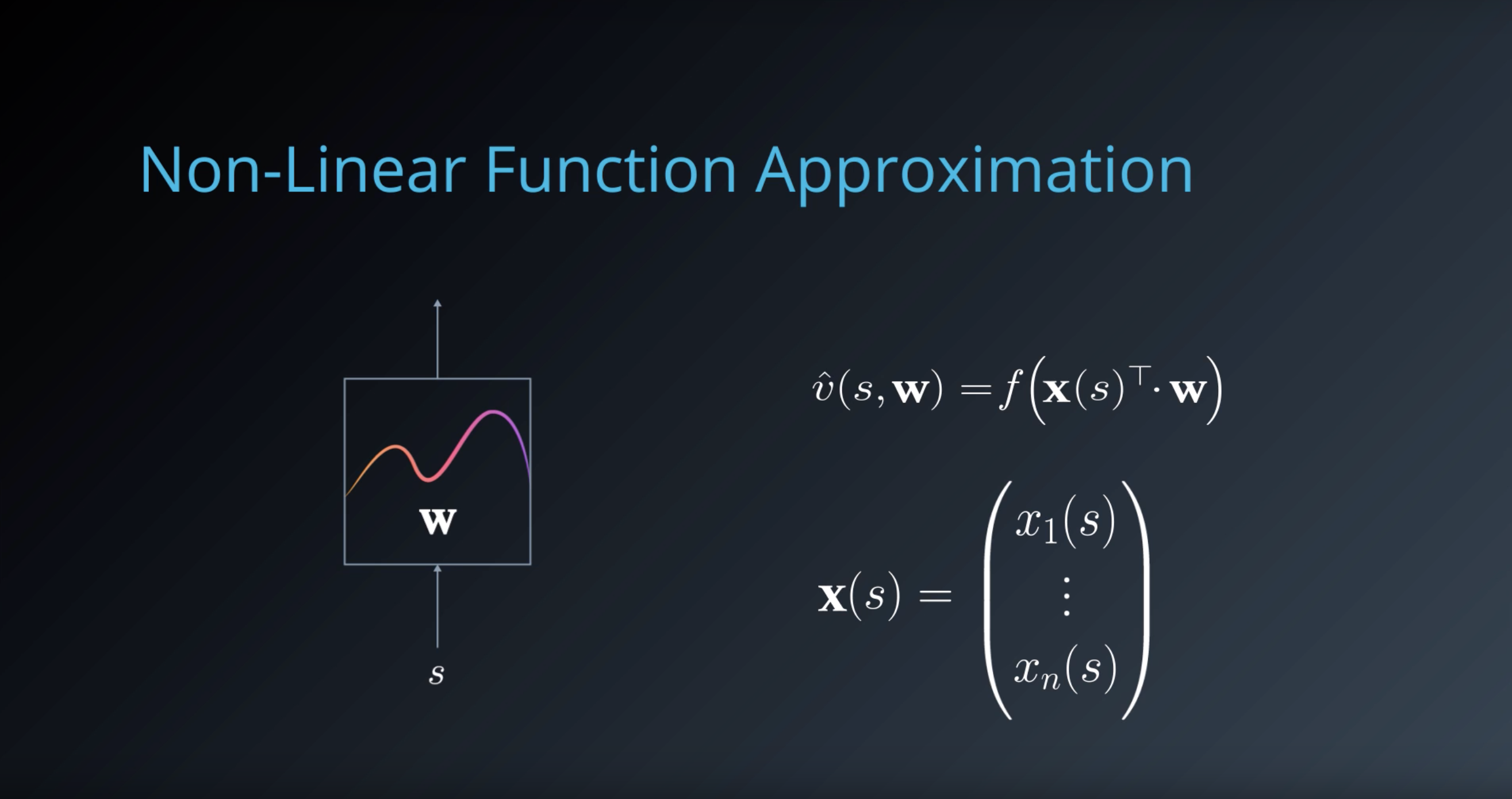
Given a problem domain with continuous states s∈S=Rn, we wish to find a way to represent the value function vπ(s) (for prediction) or qπ(s,a) (for control).

We can do this by choosing a parameterized function that approximates the true value function:

• v^(s,w)≈vπ(s)
• q^(s,a,w)≈qπ(s,a)

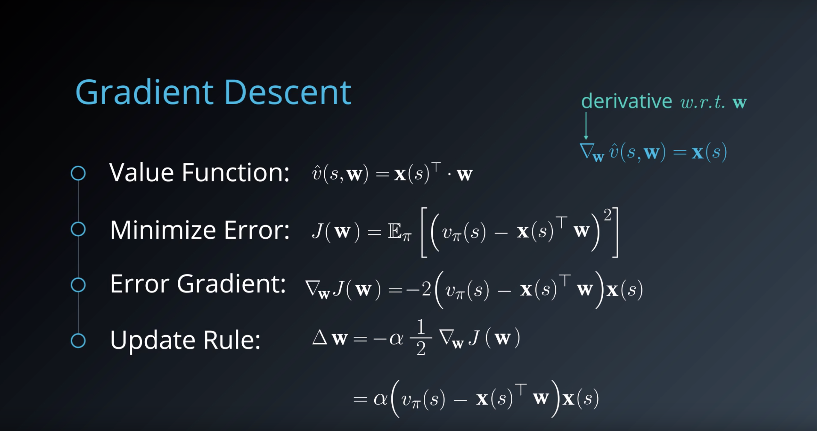
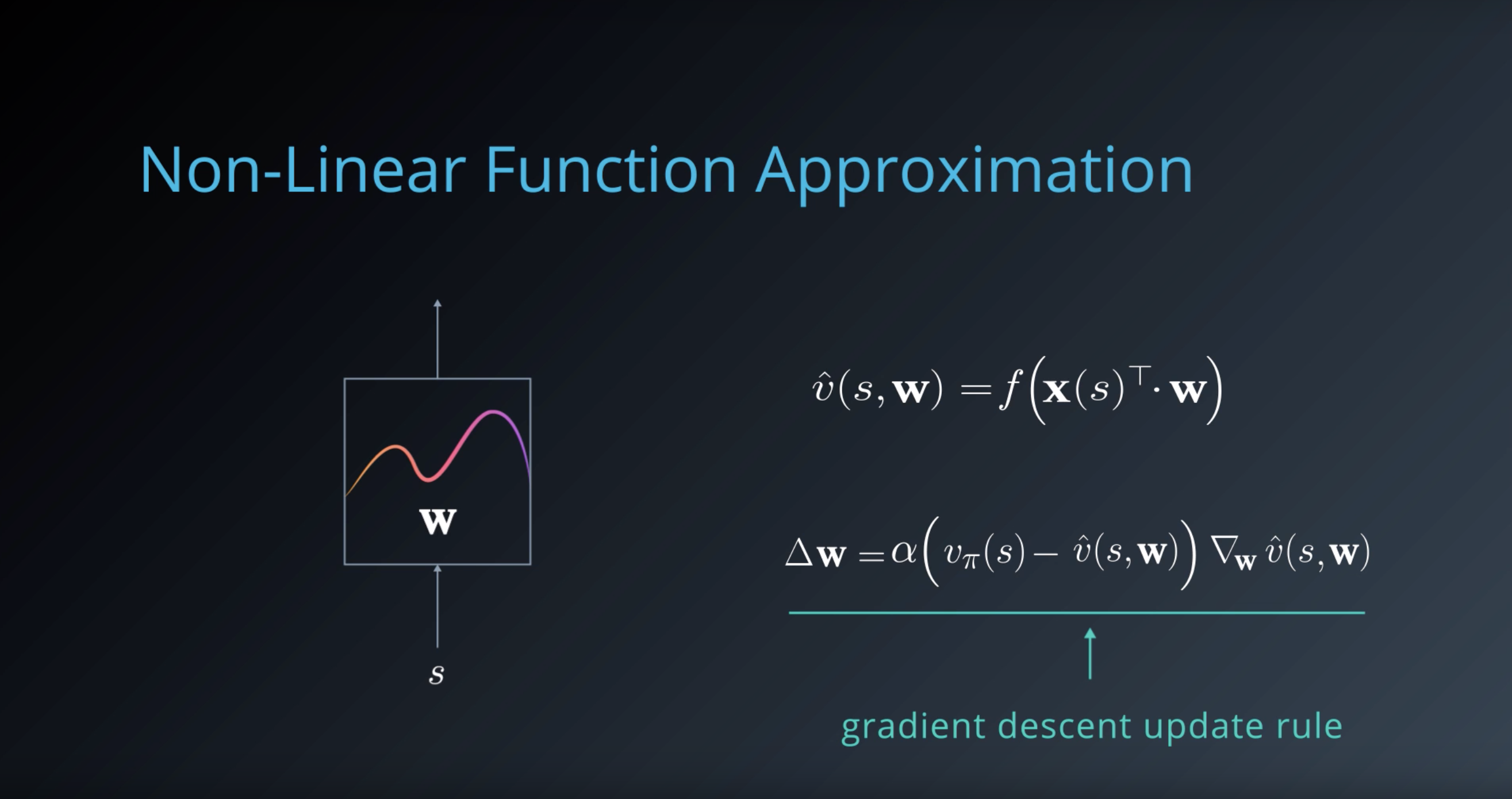
Our goal then reduces to finding a set of parameters w that yield an optimal value function. We can use the general reinforcement learning framework, with a Monte-Carlo or Temporal-Difference approach, and modify the update mechanism according to the chosen function.

Feature Vectors

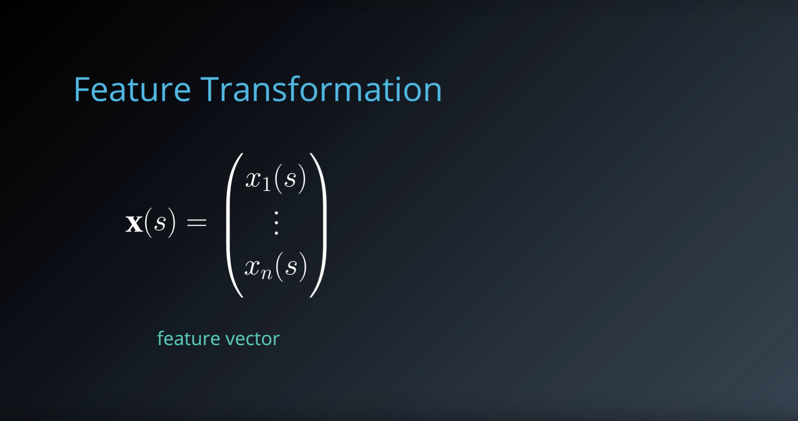
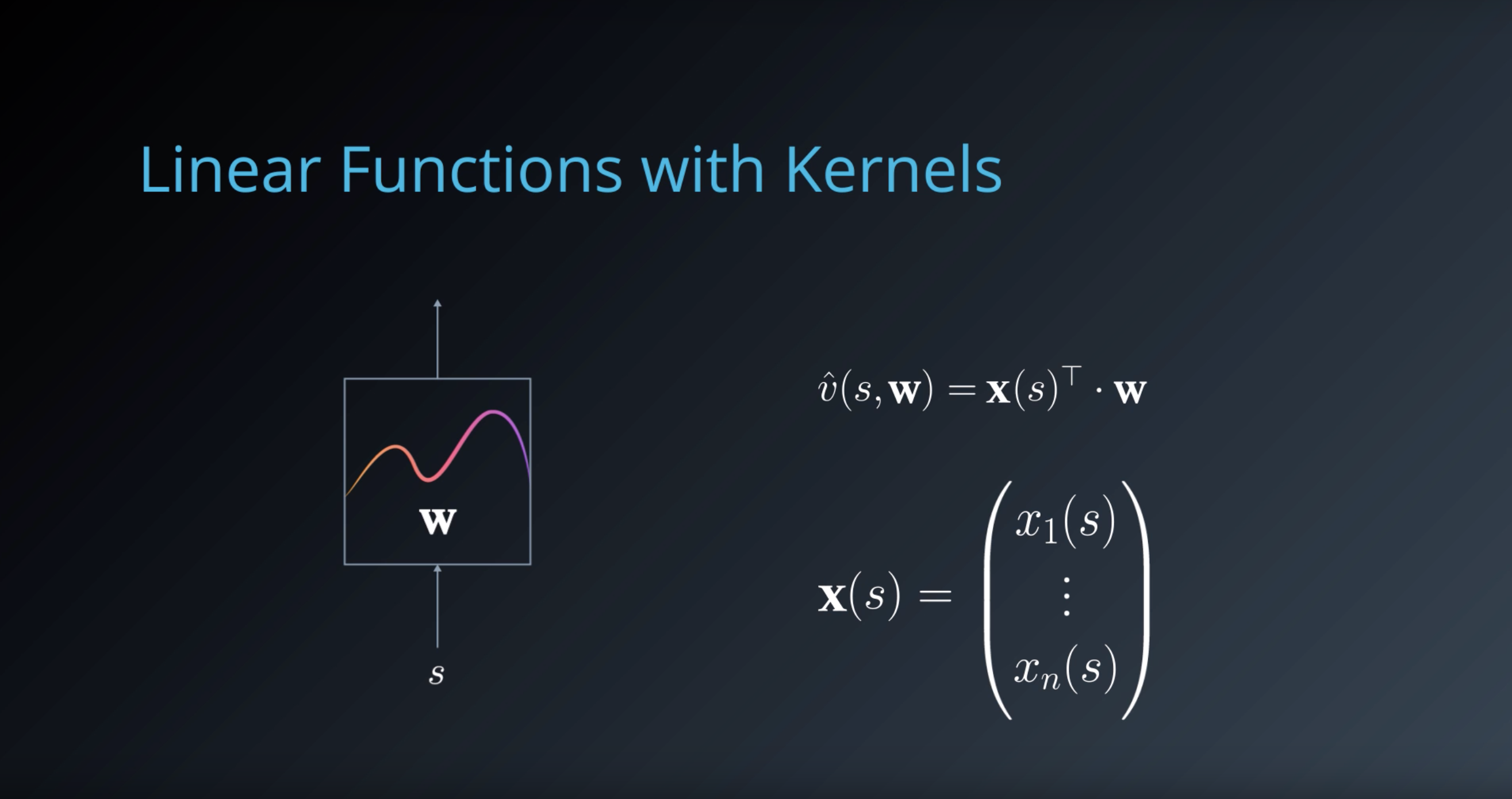
A common intermediate step is to compute a feature vector that is representative of the state: x(s)

1-6-7 : Linear Function Approximation

from IPython.display import Image
Image(filename='./images/1-6-7-1_lfa_how_would_you_tweak_w_to_bring_the_approximation_closer_to_the_true_function.png')

from IPython.display import Image
Image(filename='./images/1-6-7-2_lfa_gradient_descent.png')

from IPython.display import Image
Image(filename='./images/1-6-7-2-1_error-gradient-derivation.jpg')

from IPython.display import Image
Image(filename='./images/1-6-7-3_lfa_gradient_descent_intuition.png')

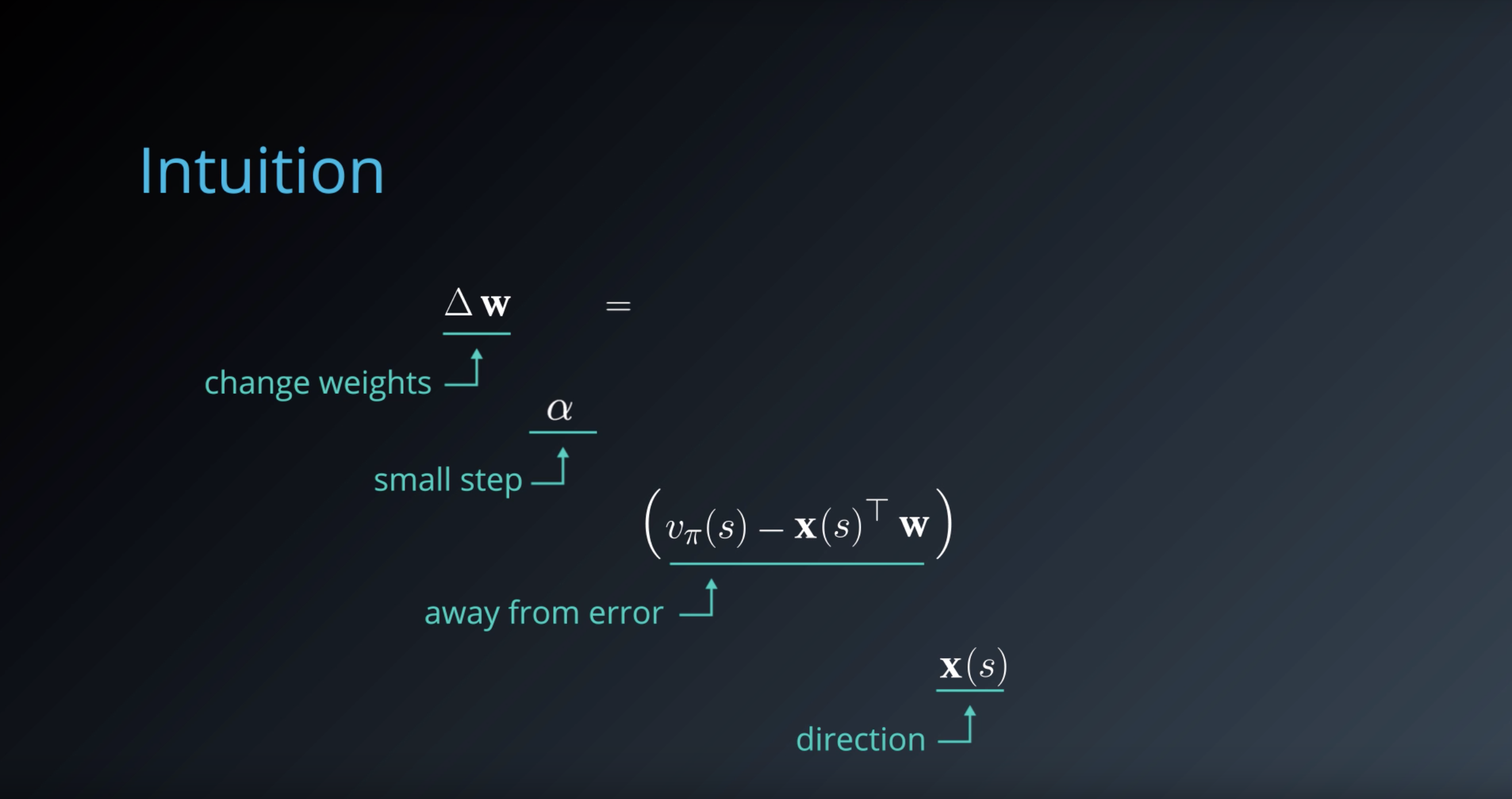
from IPython.display import Image
Image(filename='./images/1-6-7-4_lfa_action_value_approximation.png')

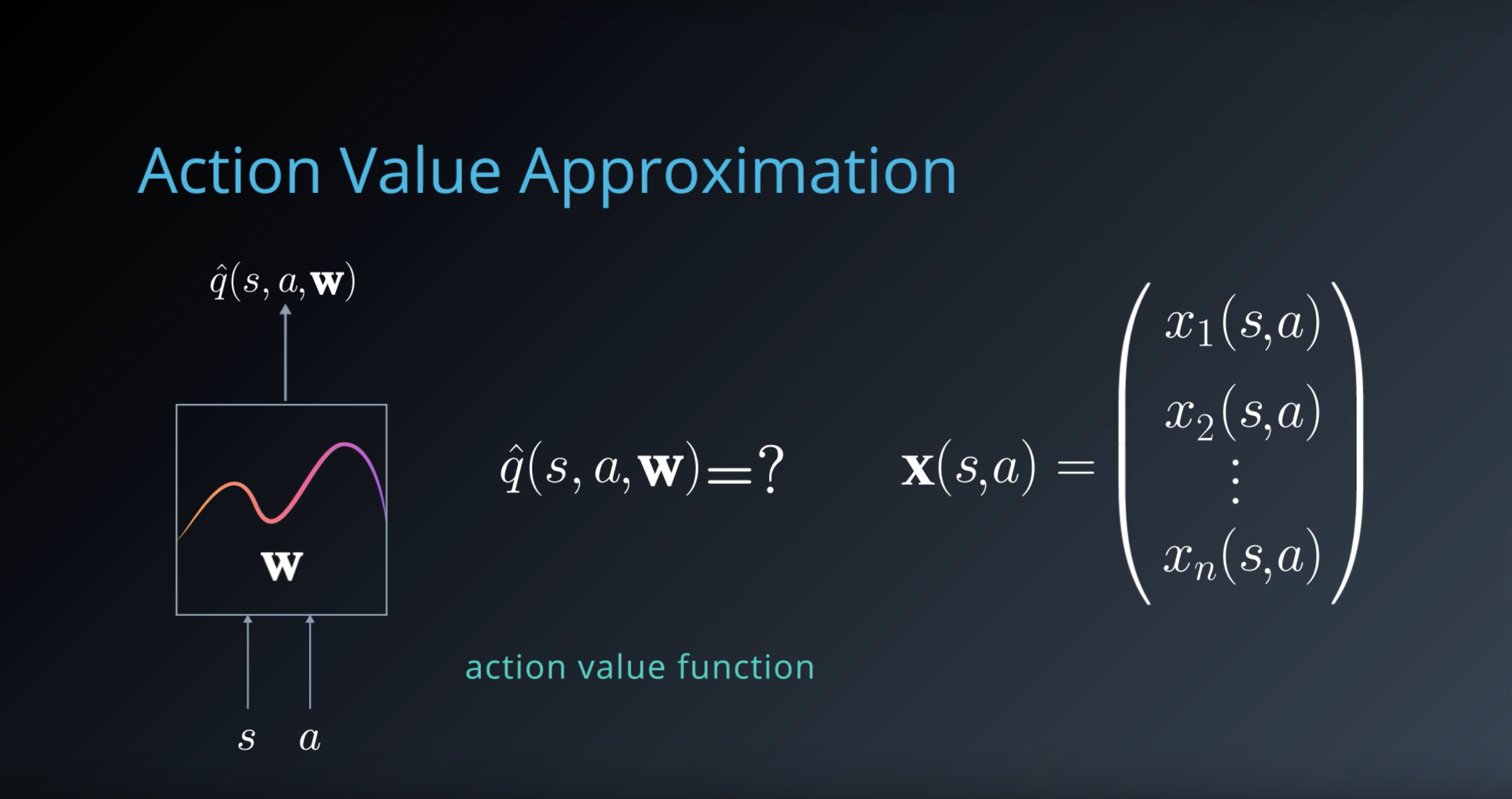
from IPython.display import Image
Image(filename='./images/1-6-7-5_lfa_action_vector_approximation.png')

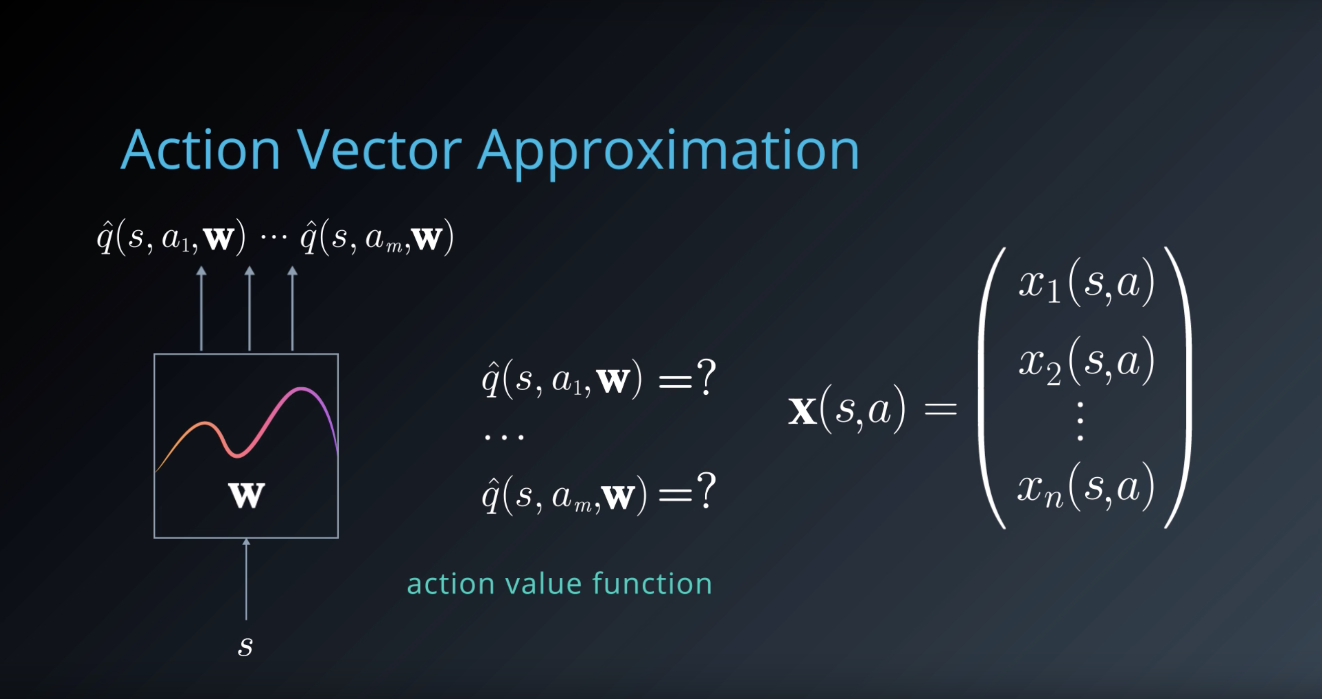
from IPython.display import Image
Image(filename='./images/1-6-7-6_lfa_action_vector_approximation.png')

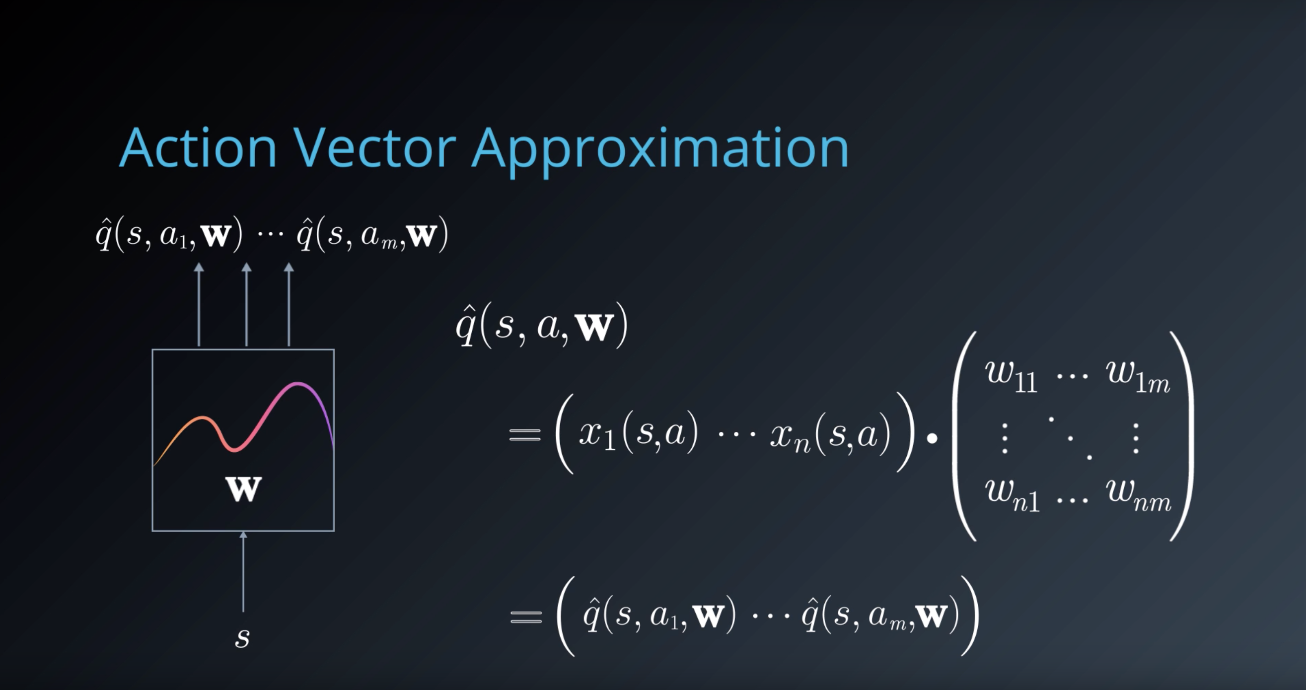
from IPython.display import Image
Image(filename='./images/1-6-7-7_lfa_limitations.png')

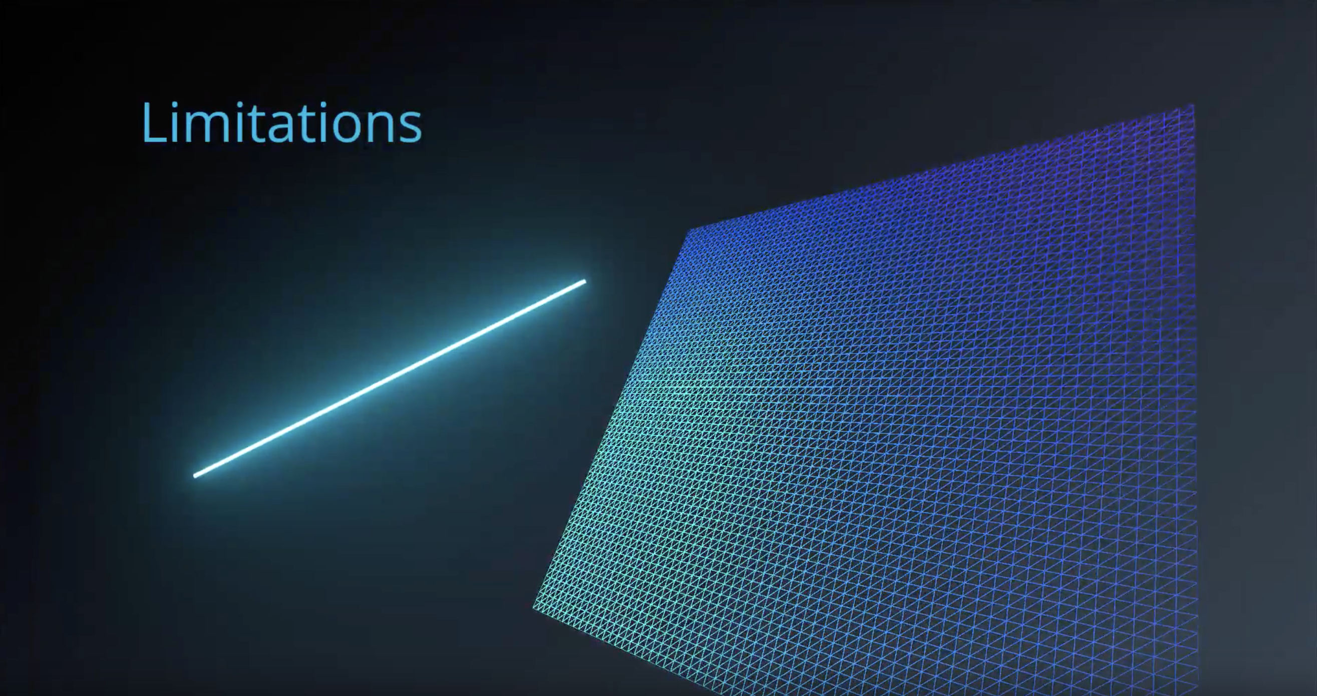
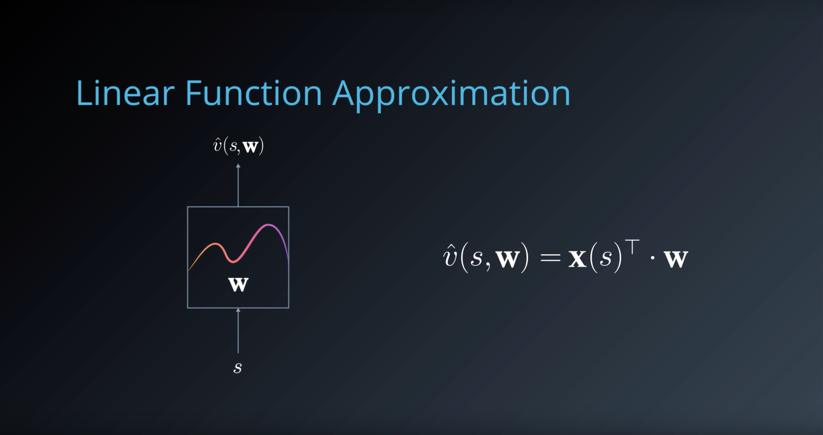
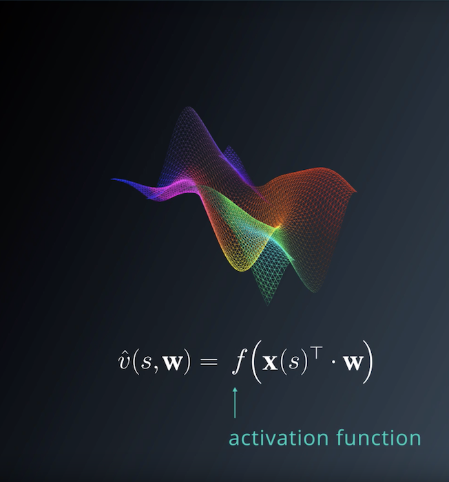
The primary limitation of linear function approximation is that we can only represent linear relationships between inputs and outputs.

1-6-8 : Kernel Functions

from IPython.display import Image
Image(filename='./images/1-6-8-1_kernel-functions_feature-transformation_takes_state_or_state-action_pair_and_produce_feature_vector.png')

from IPython.display import Image
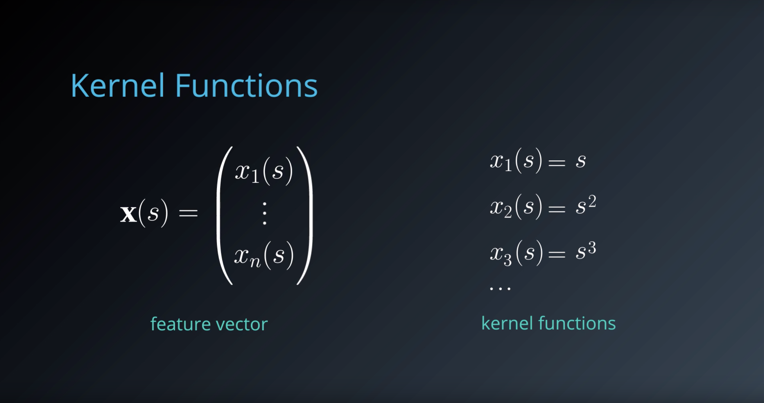
Image(filename='./images/1-6-8-2_kernel-functions_transform_the_input_state_into_a_different_space.png')

from IPython.display import Image
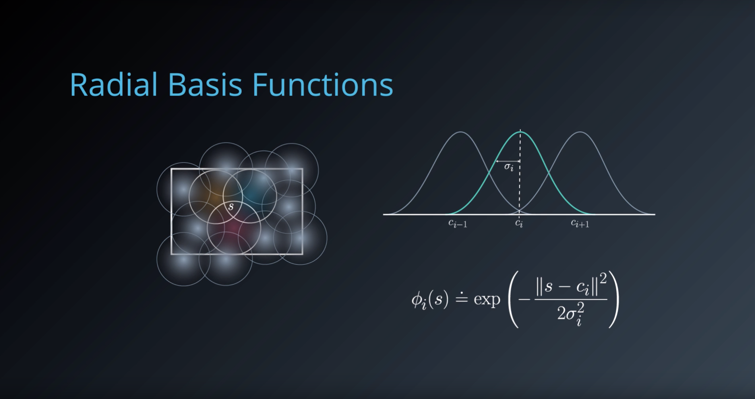
Image(filename='./images/1-6-8-3_we_can_reduce_state_representation_to_a_vector_of_responses_from_Radial-Basis-Functions.png')

1-6-9 : Non-Linear Function Approximation

from IPython.display import Image
Image(filename='./images/1-6-9-1_in_linear-functions-with-kernels_our_output_value_is_still_linear_with_respect_to_the_features.png')

from IPython.display import Image
Image(filename='./images/1-6-9-2_lets_linear_function_through_some_nonlinear_function_f_to_capture_complex_relations.png')

from IPython.display import Image
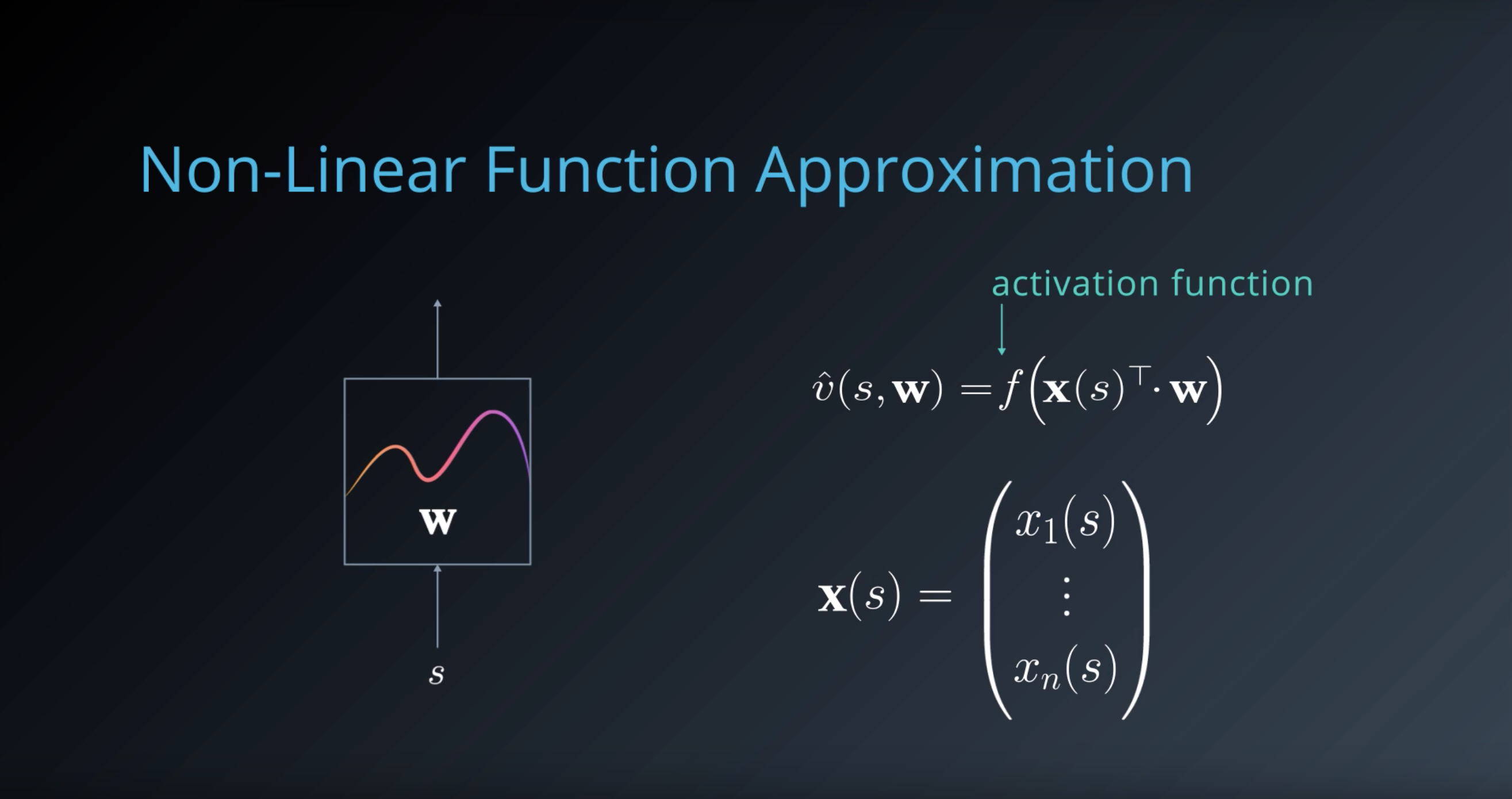
Image(filename='./images/1-6-9-3_such_a_non-linear_function_is_generally_called_an_activation_function.png')

from IPython.display import Image
Image(filename='./images/1-6-9-4_gradient_descent_update_rule.png')

1-6-10 : Summary of ‘RL in Continuous Spaces’

from IPython.display import Image
Image(filename='./images/1-6-10-1_summary_traditional-rl_use_finite-MDP_to_model.png')

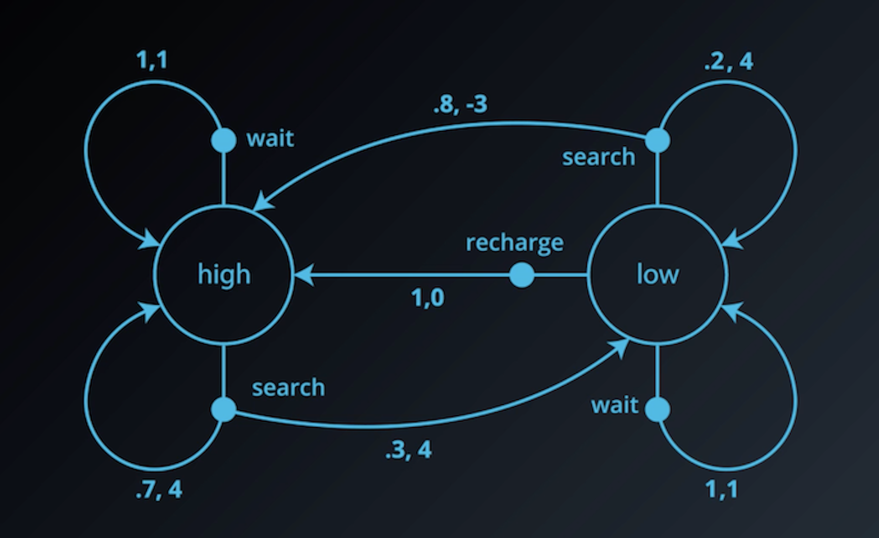
from IPython.display import Image
Image(filename='./images/1-6-10-2_summary_traditional-rl_use_finite-MDP_to_model_an_ENV_which_limits_us_to_ENV_with_discrete_state_and_action_spaces.png')

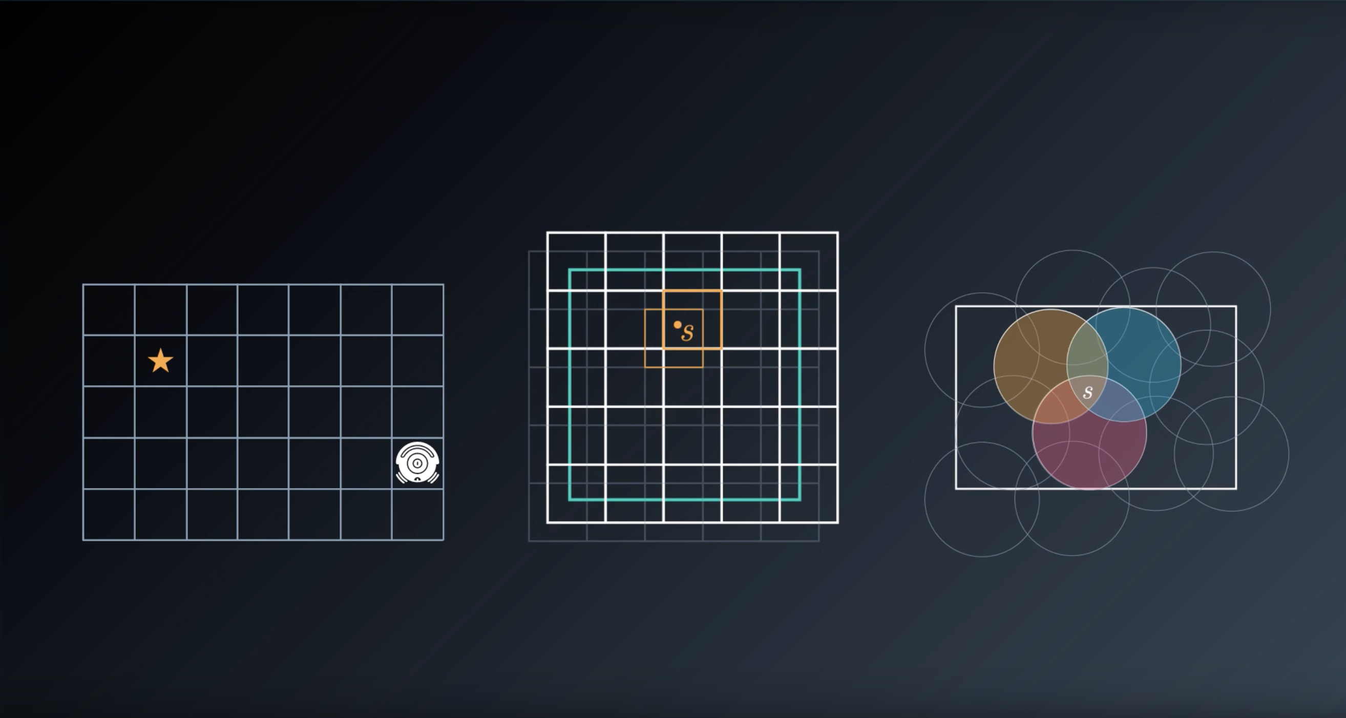
from IPython.display import Image
Image(filename='./images/1-6-10-3_summary_direct_approximation_of_value_function_compared_with_indirect_approximation_using_tile-coding_coarse-coding.png')

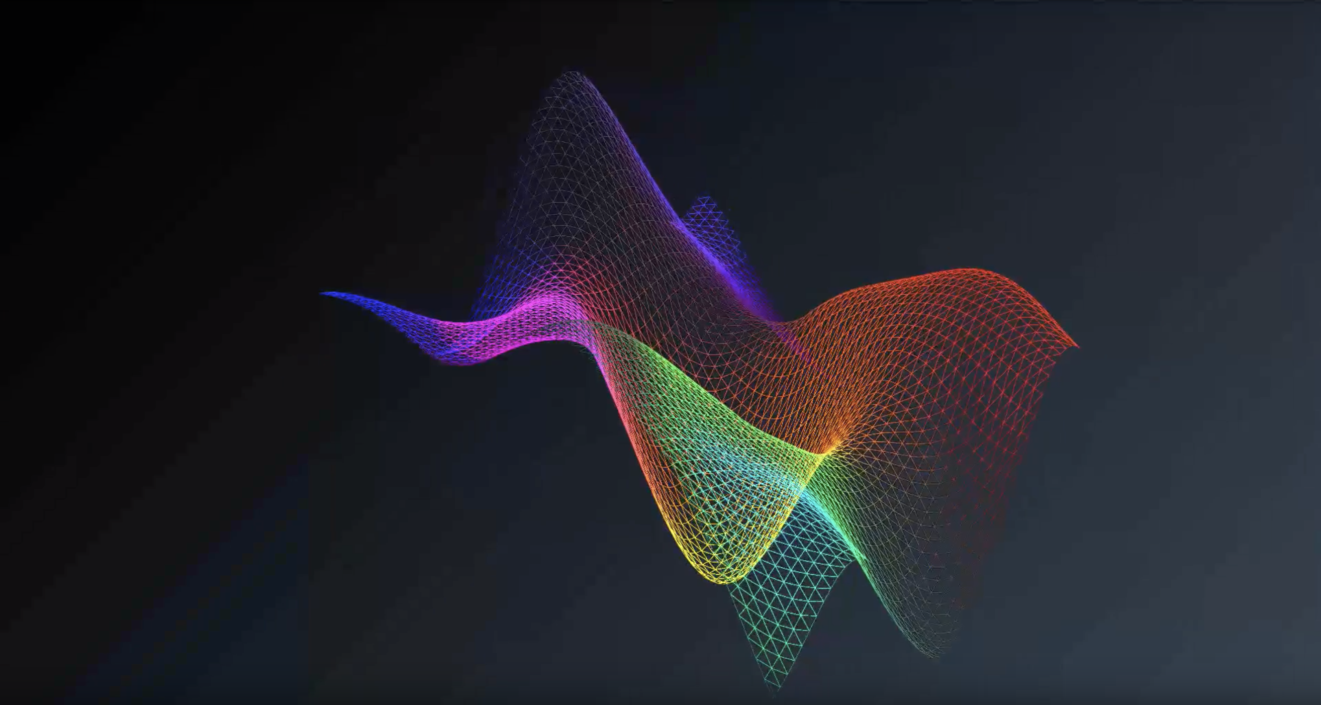
from IPython.display import Image
Image(filename='./images/1-6-10-4_summary_defining_feature-transformation_then_computing_a_linear-combination_of_features_by_non-linear_feature-transforms_like_Radial-Basis-Functions.png')

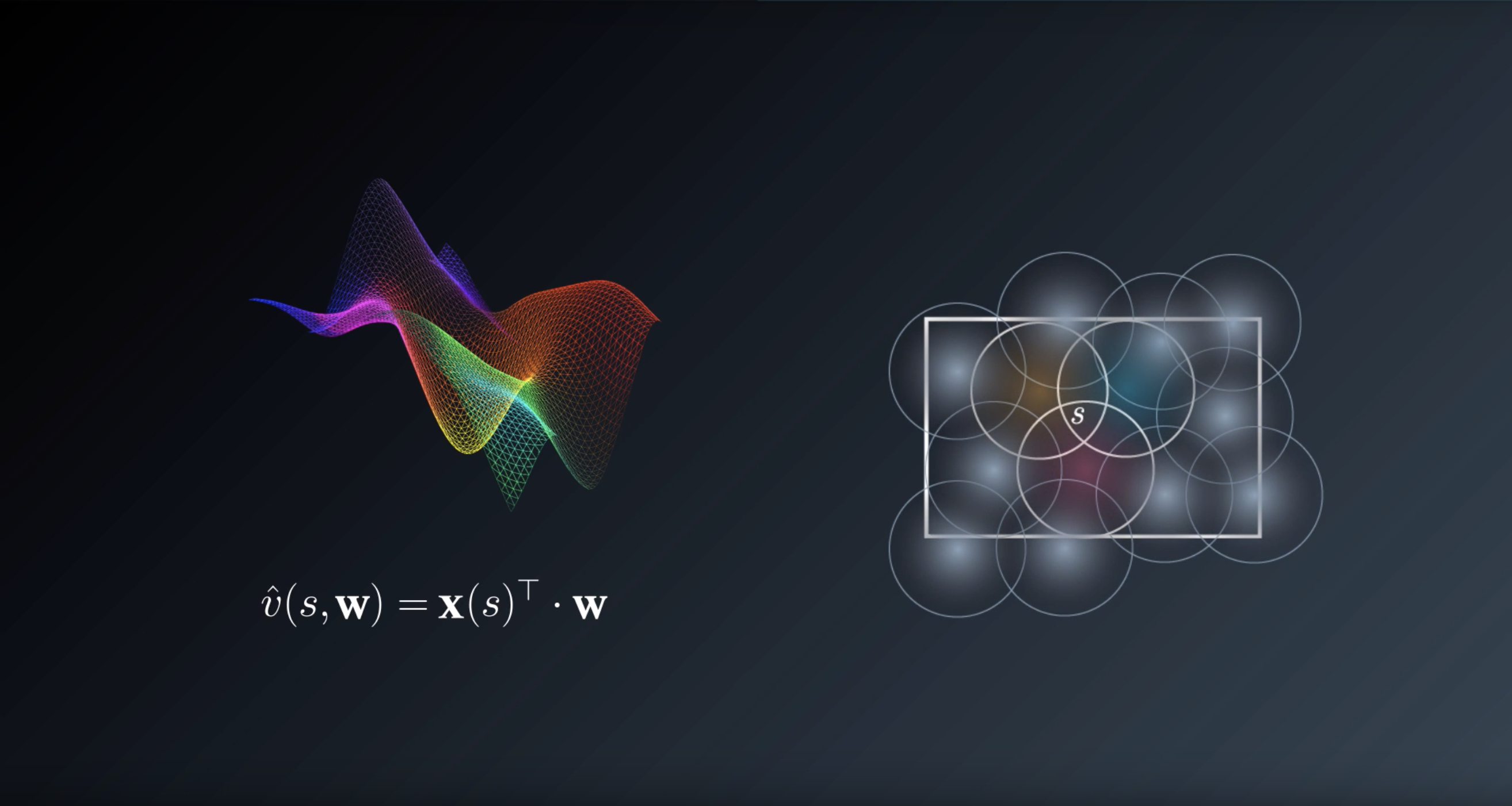
from IPython.display import Image
Image(filename='./images/1-6-10-5_summary_to_represent_non-linear_relationships_across_combinagtions_of_features_we_can_use_activagtion_function.png')