DRL Introduction

from IPython.display import Image
Image(filename='./images/1-0-0-0_opening.jpg')

Learning Plan

Lesson 1-0: Introduction to RL

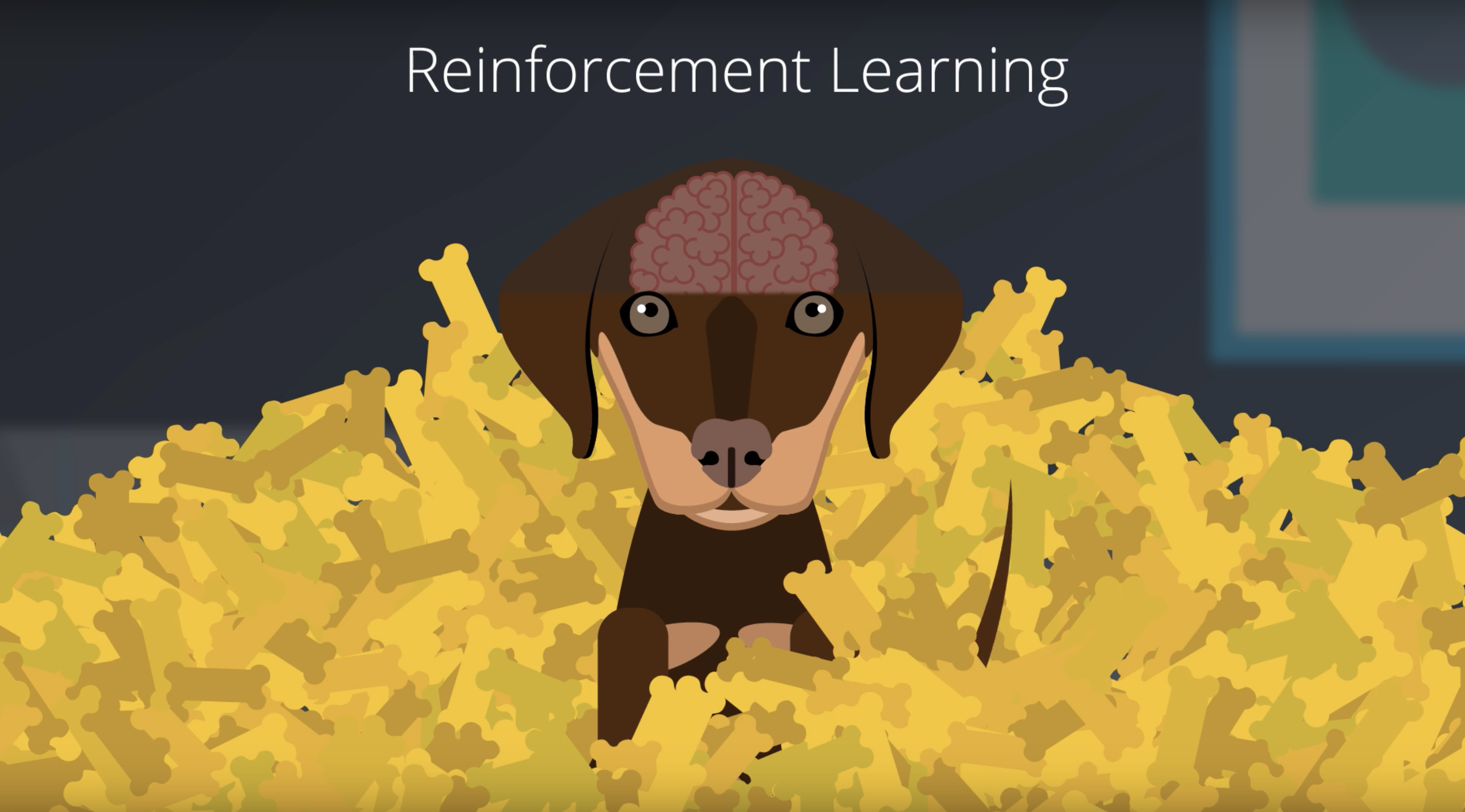
In this lesson, you’ll explore a friendly introduction to reinforcement learning.

Lesson 1-1: The RL Framework: The Problem

In this lesson, you’ll learn how to specify a real-world problem as a Markov Decision Process (MDP), so that it can be solved with reinforcement learning.

Lesson 1-2: The RL Framework: The Solution

In this lesson, you’ll learn all about value functions and optimal policies.

Lesson 1-3: Dynamic Programming (Optional)

In this lesson, you’ll build some intuition for the reinforcement learning problem by learning about a class of solution methods that solve a slightly easier problem. (This lesson is optional and can be accessed in the extracurricular content.)

Lesson 1-4: Monte Carlo Methods

In this lesson, you’ll learn about a class of solution methods known as Monte Carlo methods. You’ll implement your own Blackjack-playing agent in OpenAI Gym

Lesson 1-5: Temporal-Difference Methods

In this lesson, you’ll learn how to apply temporal-difference methods such as SARSA, Q-learning, and Expected SARSA to solve both episodic and continuing tasks.

Lesson 1-6: Solve OpenAI Gym’s Taxi-v2 Task

In this lesson, you’ll apply what you’ve learned to train a taxi to pick up and drop off passengers.

Lesson 1-7: RL in Continuous Spaces

In this lesson, you’ll explore how to use techniques such as tile coding and coarse coding to expand the size of the problems that can be solved with traditional reinforcement learning algorithms.

Textbook

[Reinforcement Learning: An Introduction by Richard S. Sutton and Andrew G. Barto - Second Edition] http://incompleteideas.net/book/the-book.html

Lesson 1-0: Introduction to RL

1-0-1 : Introduction

from IPython.display import Image
Image(filename='./images/1-0-1-1_introduction.png')

from IPython.display import Image
Image(filename='./images/1-0-1-2_introduction.png')

from IPython.display import Image
Image(filename='./images/1-0-1-3_introduction.png')

from IPython.display import Image
Image(filename='./images/1-0-1-4_introduction.png')

from IPython.display import Image
Image(filename='./images/1-0-1-5_introduction.png')

1-0-2 : Applications

AlphaGo Zero

Read about AlphaGo Zero, the state-of-the-art computer program that defeats professional human Go players

from IPython.display import HTML
HTML('<iframe width="560" height="315" src="https://www.youtube.com/embed/tXlM99xPQC8" frameborder="0" allow="accelerometer; autoplay; encrypted-media; gyroscope; picture-in-picture" allowfullscreen></iframe>>')

Atari games

Learn about how reinforcement learning (RL) is used to play Atari games.

from IPython.display import HTML
HTML('<iframe width="560" height="315" src="https://www.youtube.com/embed/xN1d3qHMIEQ" frameborder="0" allow="accelerometer; autoplay; encrypted-media; gyroscope; picture-in-picture" allowfullscreen></iframe>')

OpenAI’s bot

Read about OpenAI’s bot that beat the world’s top players of Dota 2.

from IPython.display import HTML
HTML('<iframe width="560" height="315" src="https://www.youtube.com/embed/l92J1UvHf6M" frameborder="0" allow="accelerometer; autoplay; encrypted-media; gyroscope; picture-in-picture" allowfullscreen></iframe>')

Humanoid bodies to walk

Read about research used to teach humanoid bodies to walk

from IPython.display import Image
Image(filename='./images/1-0-2-1_humanoid_body_to_work.gif')

<IPython.core.display.Image object>

self-driving cars

Learn about RL for self-driving cars.

from IPython.display import HTML
HTML('<iframe width="560" height="315" src="https://www.youtube.com/embed/_OCjqIgxwHw" frameborder="0" allow="accelerometer; autoplay; encrypted-media; gyroscope; picture-in-picture" allowfullscreen></iframe>')

RL for telecommunication

Learn about RL for telecommunication.

from IPython.display import HTML
HTML('<iframe width="560" height="315" src="https://papers.nips.cc/paper/1740-low-power-wireless-communication-via-reinforcement-learning.pdf" frameborder="0" allow="accelerometer; autoplay; encrypted-media; gyroscope; picture-in-picture" allowfullscreen></iframe>')

RL for inventory management

Read this paper that introduces RL for inventory management

from IPython.display import HTML
HTML('<iframe width="560" height="315" src="http://read.pudn.com/downloads142/sourcecode/others/617477/inventory%20supply%20chain/04051310570412465(1).pdf" frameborder="0" allow="accelerometer; autoplay; encrypted-media; gyroscope; picture-in-picture" allowfullscreen></iframe>')

1-0-3 : Dog Example

from IPython.display import Image
Image(filename='./images/1-0-3-1_dog_example.png')

from IPython.display import Image
Image(filename='./images/1-0-3-2_dog_example.png')

from IPython.display import Image
Image(filename='./images/1-0-3-3_dog_example.png')

from IPython.display import Image
Image(filename='./images/1-0-3-4_dog_example.png')

from IPython.display import Image
Image(filename='./images/1-0-3-5_dog_example.png')

from IPython.display import Image
Image(filename='./images/1-0-3-6_dog_example.png')

from IPython.display import Image
Image(filename='./images/1-0-3-7_dog_example.png')

from IPython.display import Image
Image(filename='./images/1-0-3-8_dog_example.png')

from IPython.display import Image
Image(filename='./images/1-0-3-9_dog_example.png')

Lesson 1-1: The RL Framework: The Problem

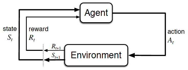
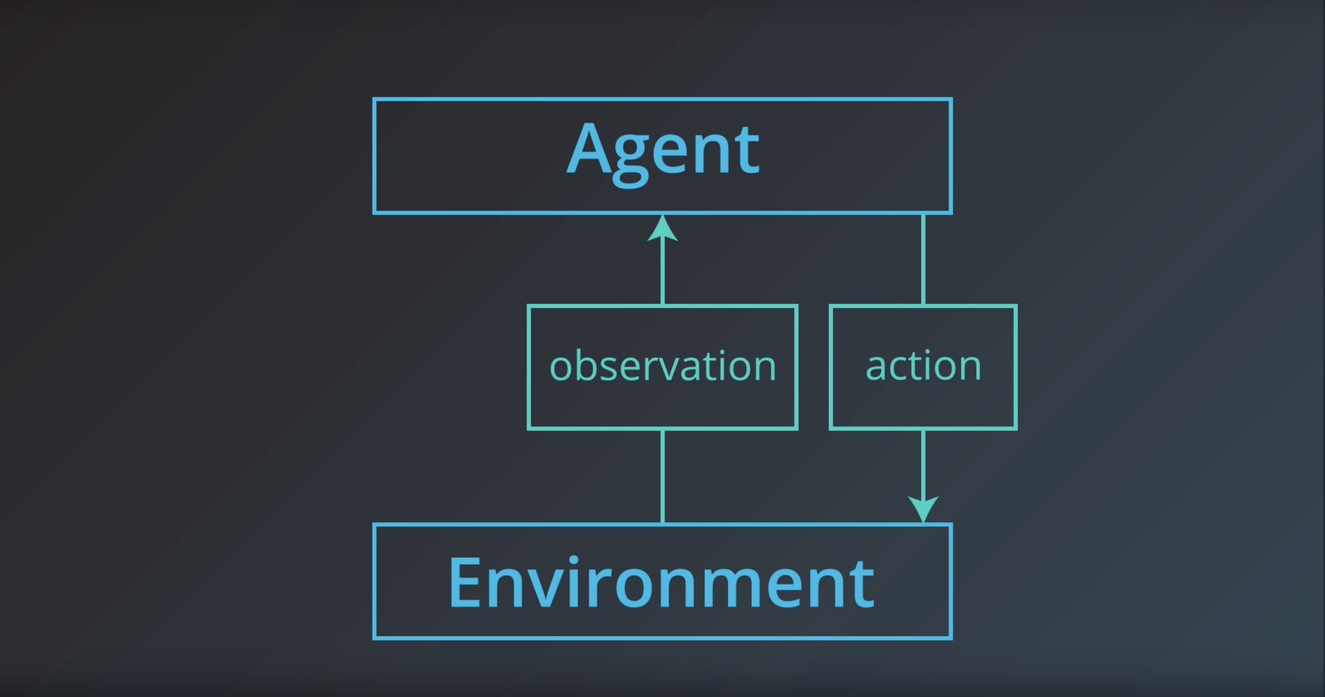
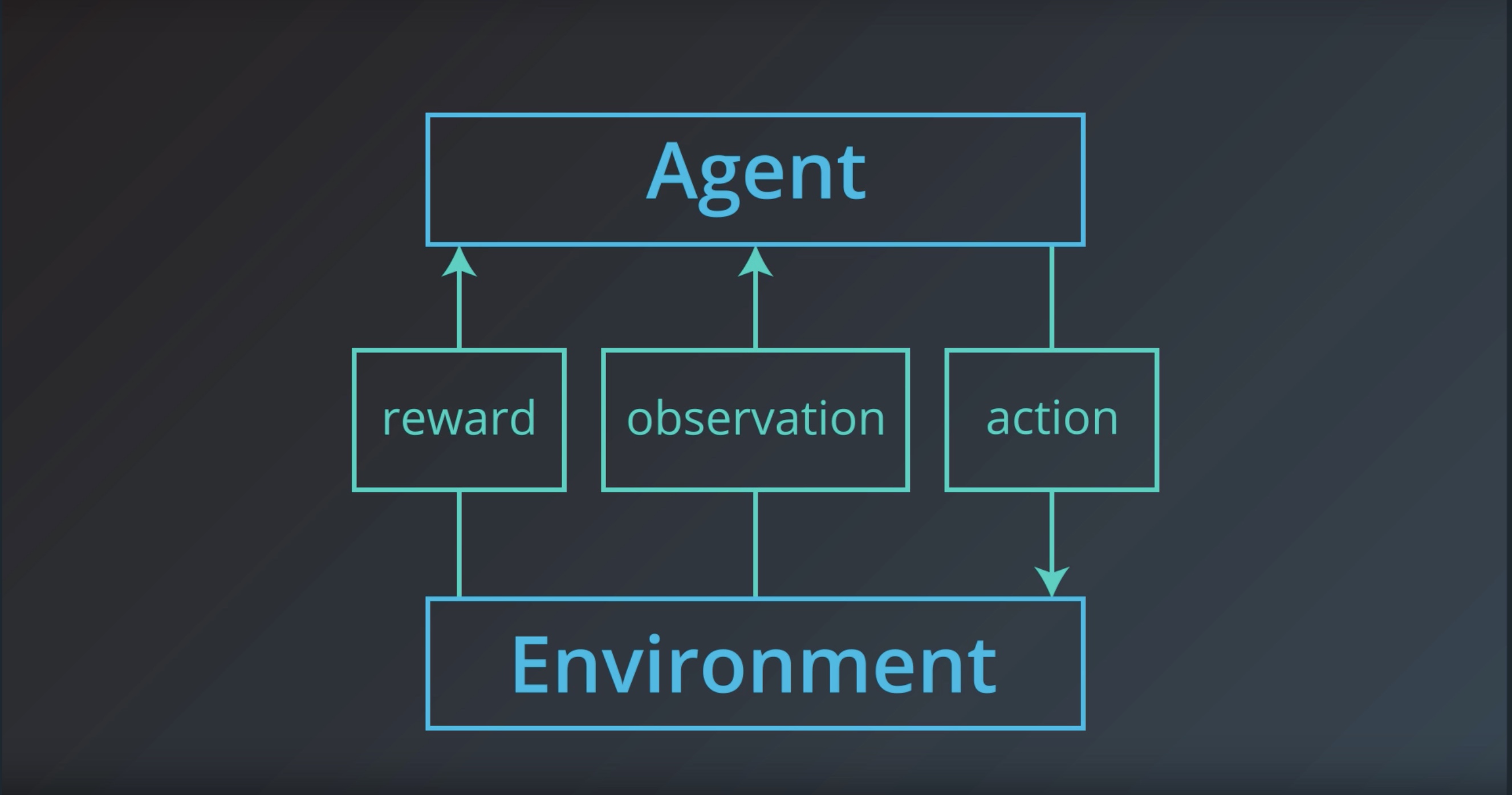
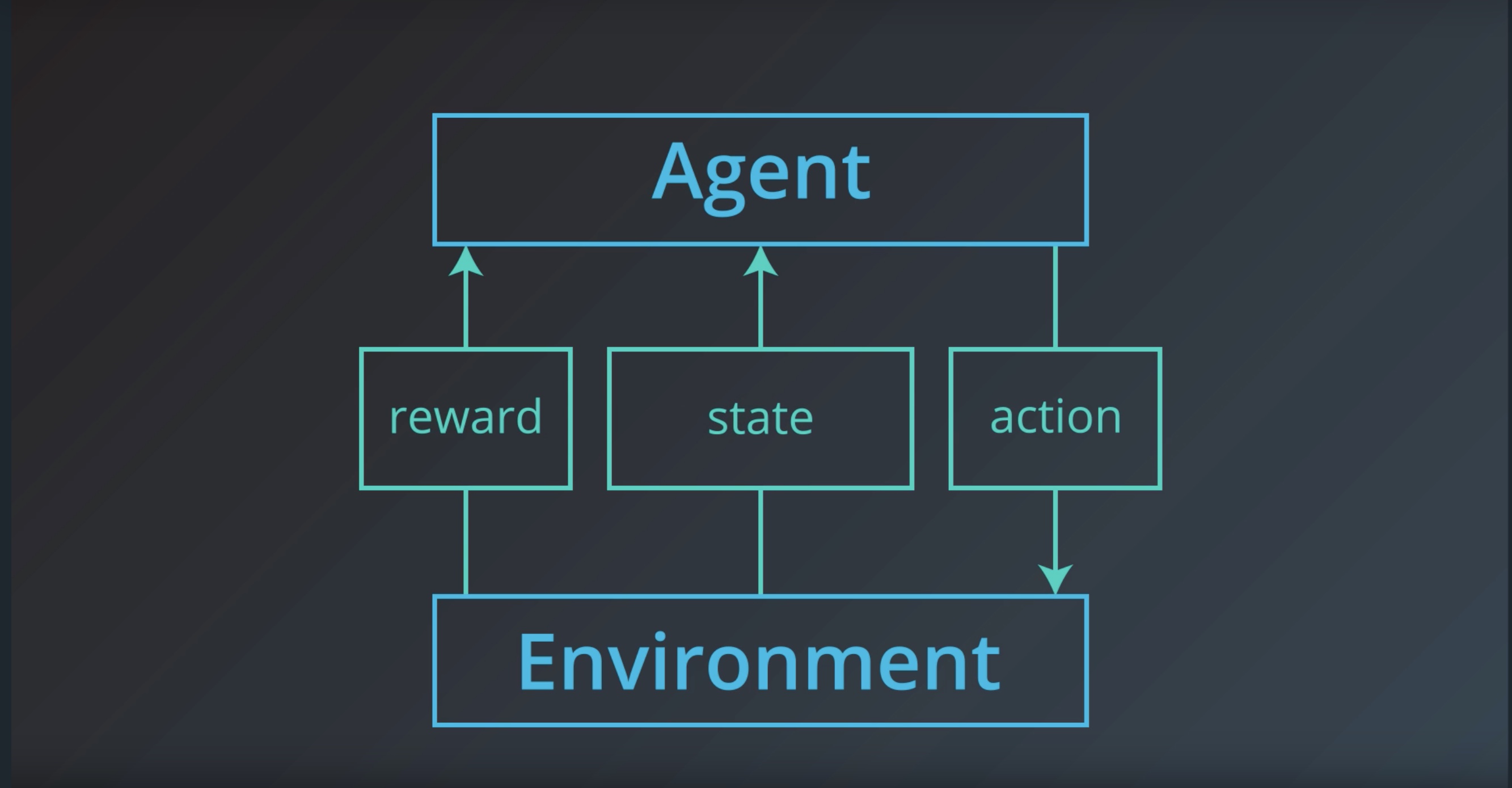
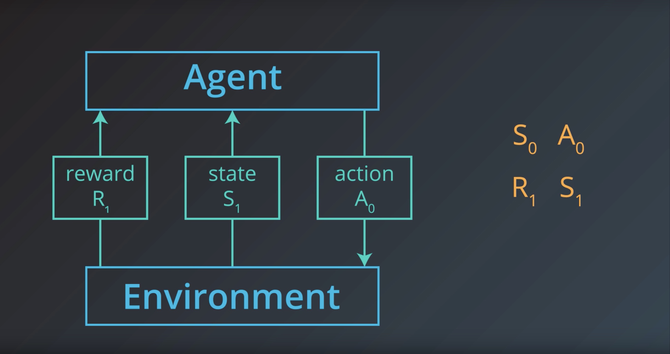
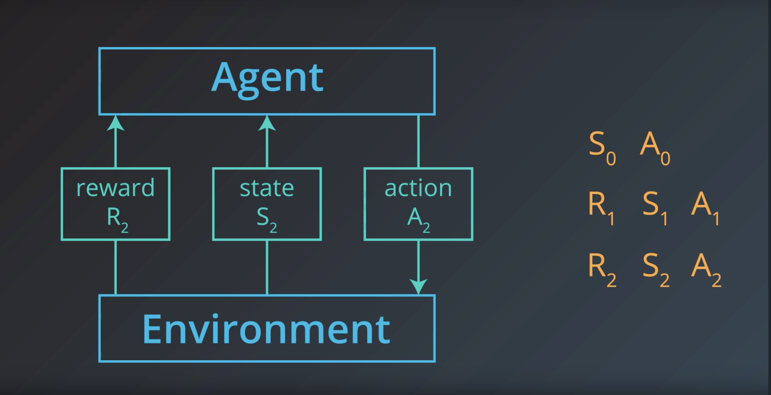
1-1-1 : RL Framework Basic Concepts

• agent
• envirionment
• state
• action
• reward

from IPython.display import Image
Image(filename='./images/1-1-1-0_agent_environment_interaction_in_rl-Sutton_Barto_2017.png')

from IPython.display import Image
Image(filename='./images/1-1-1-1_agent.jpeg')

from IPython.display import Image
Image(filename='./images/1-1-1-2_environment.jpeg')

from IPython.display import Image
Image(filename='./images/1-1-1-3_observation.jpeg')

Observation = a situation that the environment presents to the agent

from IPython.display import Image
Image(filename='./images/1-1-1-4_action.jpeg')

from IPython.display import Image
Image(filename='./images/1-1-1-5_reward.jpeg')

from IPython.display import Image
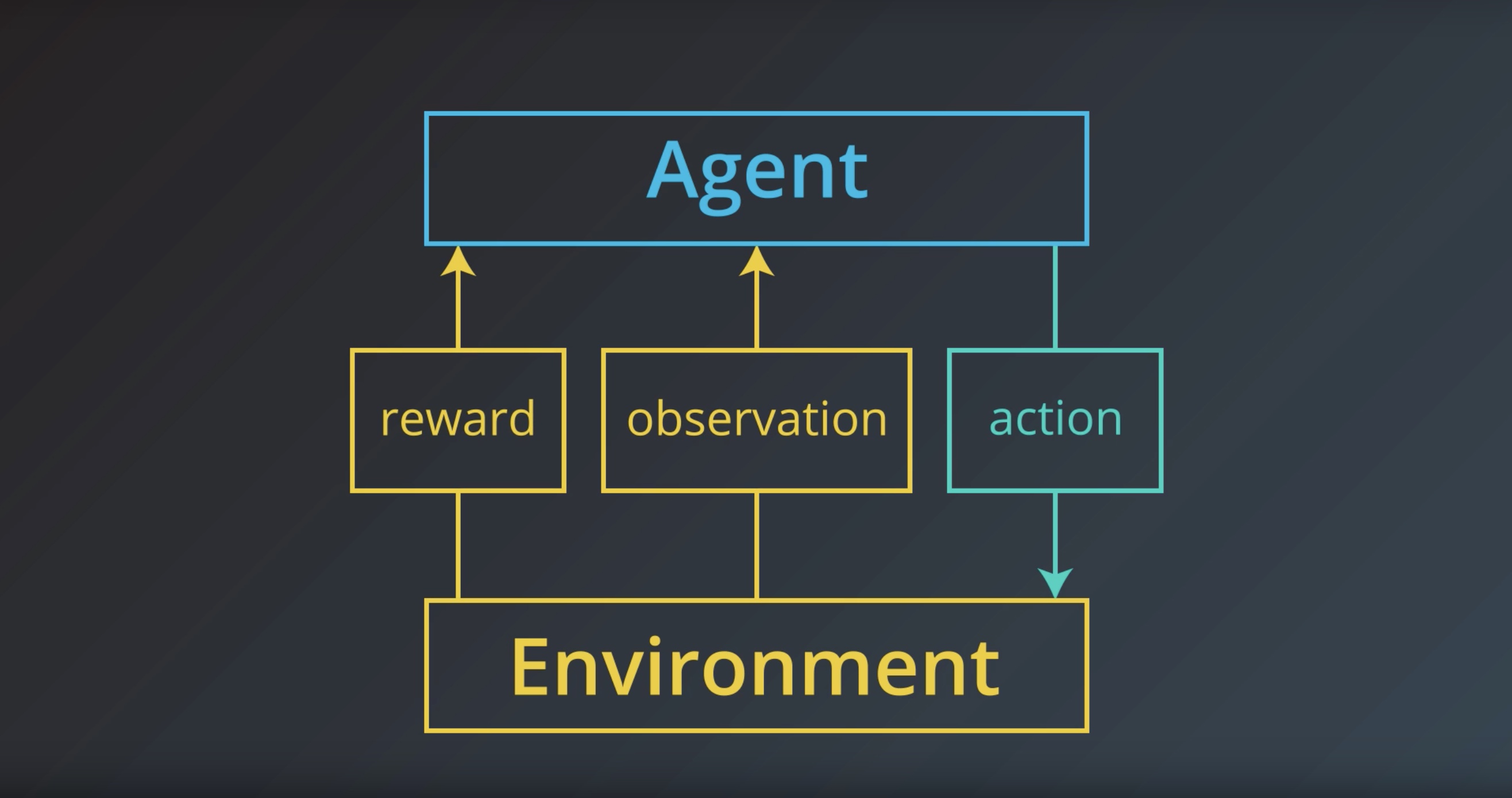
Image(filename='./images/1-1-1-6_environment_sends_observation_and_reward.jpeg')

from IPython.display import Image
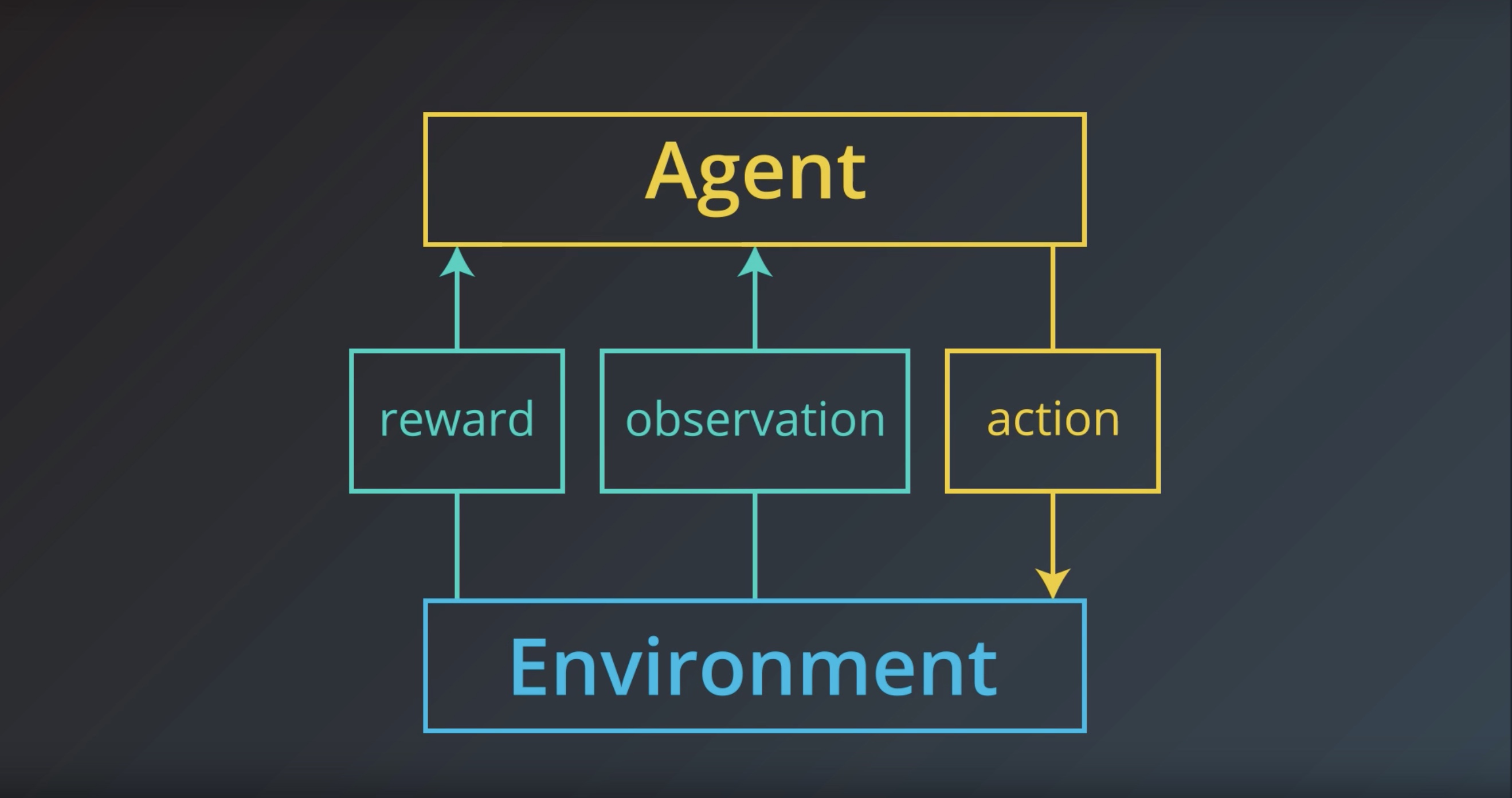
Image(filename='./images/1-1-1-7_agent_choose_an_action.jpeg')

In general, we don’t need to assume that …

the environment shows the agent everything he needs to make well-informed decisions.

from IPython.display import Image
Image(filename='./images/1-1-1-8_agent_receive_the_environment_state.jpeg')

But ite greatly simplifies the underlying mathematics…

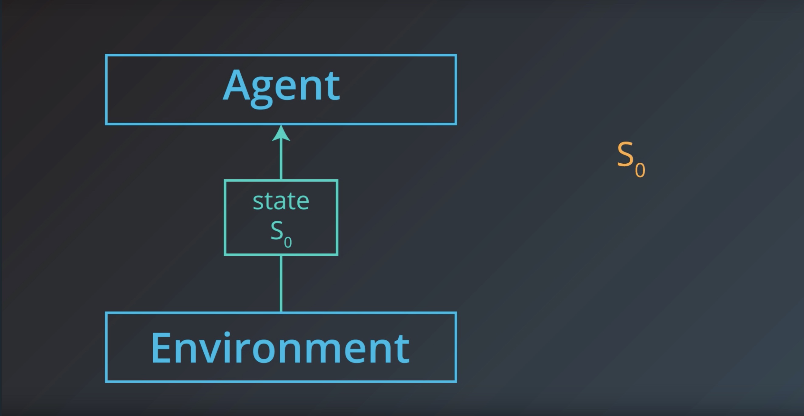
We’ll make the assumption that the agent is able to fully observe what ever state the environment is in.

And instead of referring to the agent as receiveing an obervagtion,

The agent receives the enviroment state

from IPython.display import Image
Image(filename='./images/1-1-1-9_state0.jpeg')

from IPython.display import Image
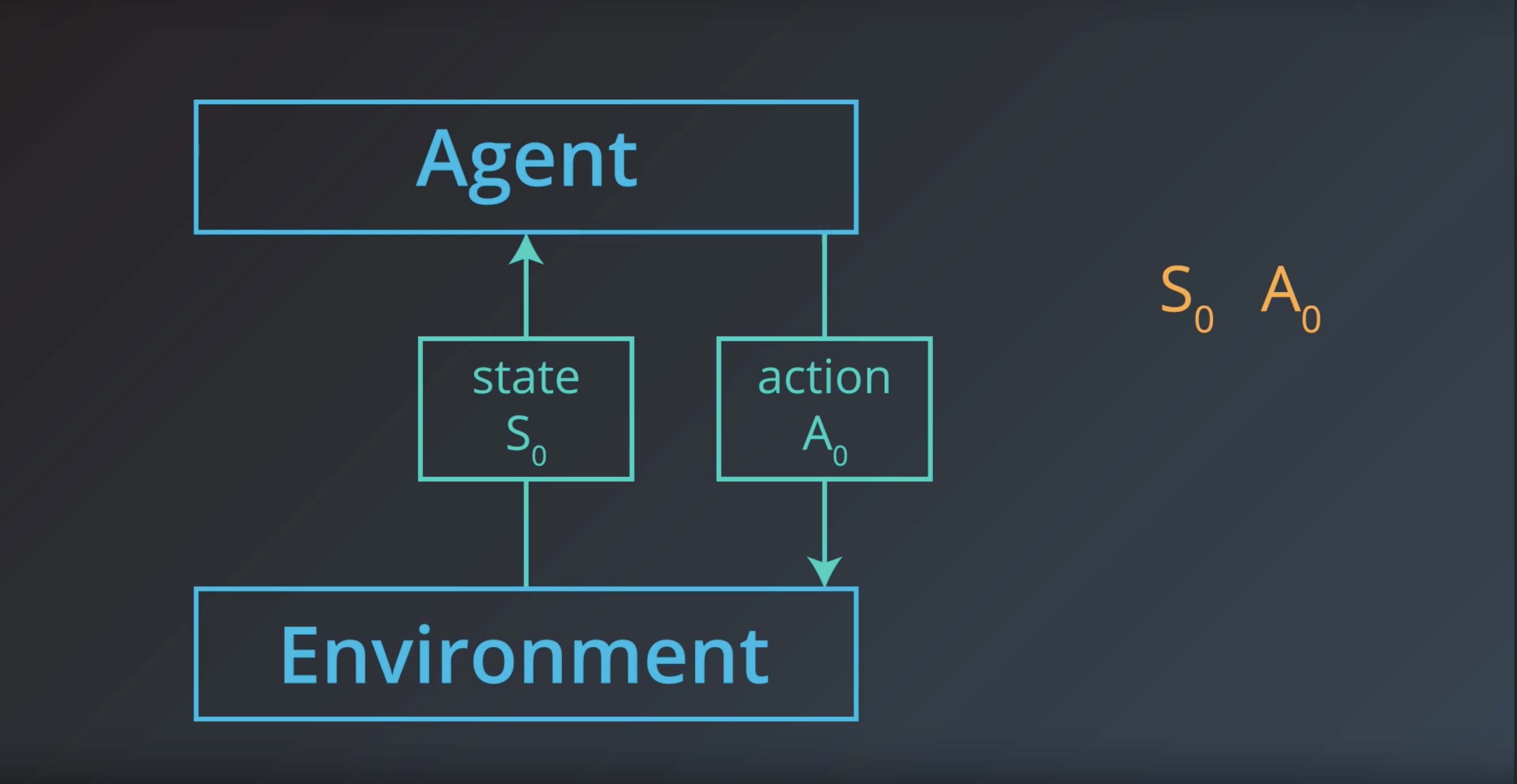
Image(filename='./images/1-1-1-10_action0.jpeg')

from IPython.display import Image
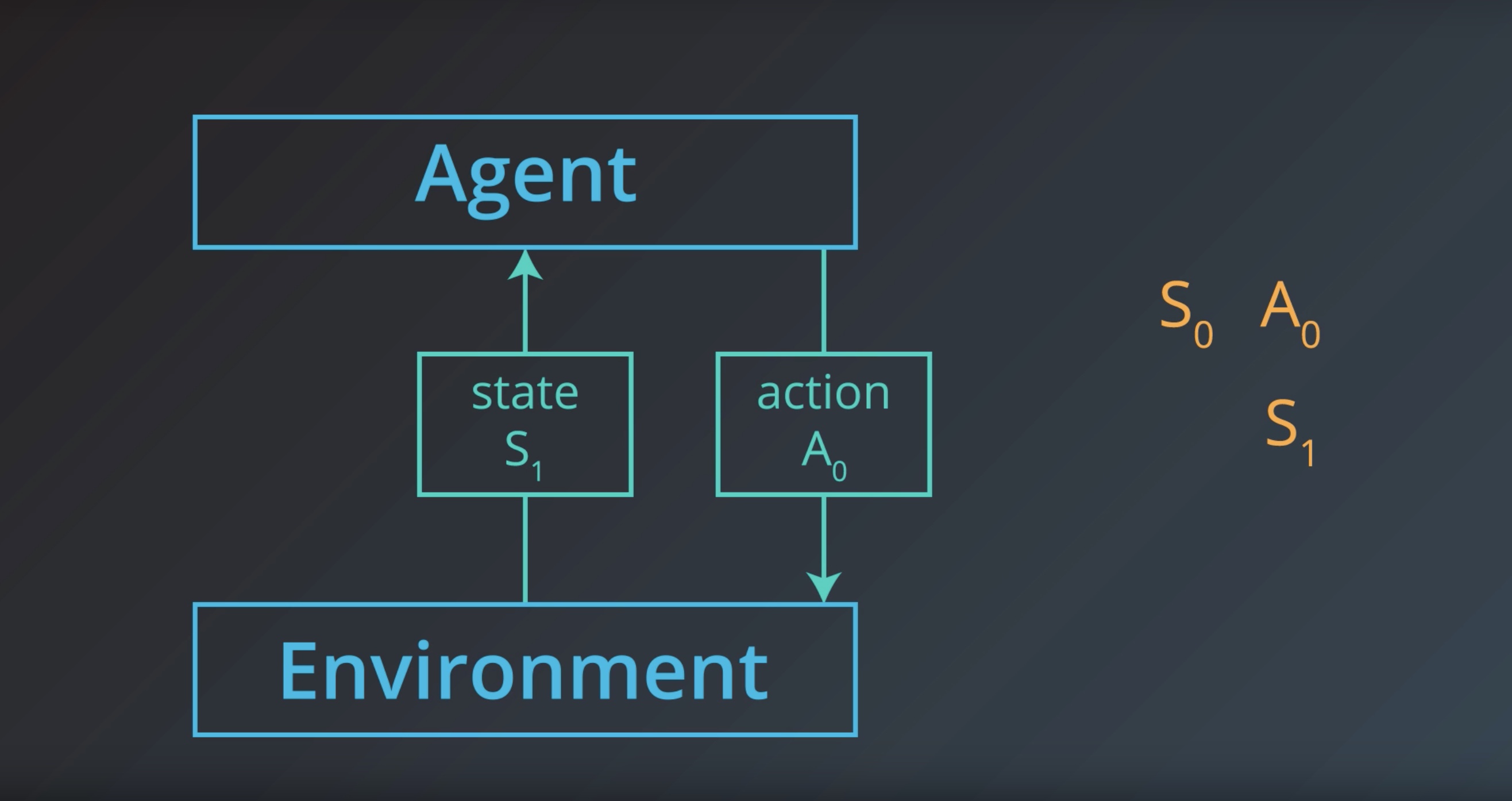
Image(filename='./images/1-1-1-11_state1.jpeg')

from IPython.display import Image
Image(filename='./images/1-1-1-12_reward1.jpeg')

from IPython.display import Image
Image(filename='./images/1-1-1-13_interaction_between_agent_and_environemnt.jpeg')

from IPython.display import Image
Image(filename='./images/1-1-1-14_interaction_is_sequence_of_sar.jpeg')

from IPython.display import Image
Image(filename='./images/1-1-1-15_maximize_expected_cumulative_reward.jpeg')

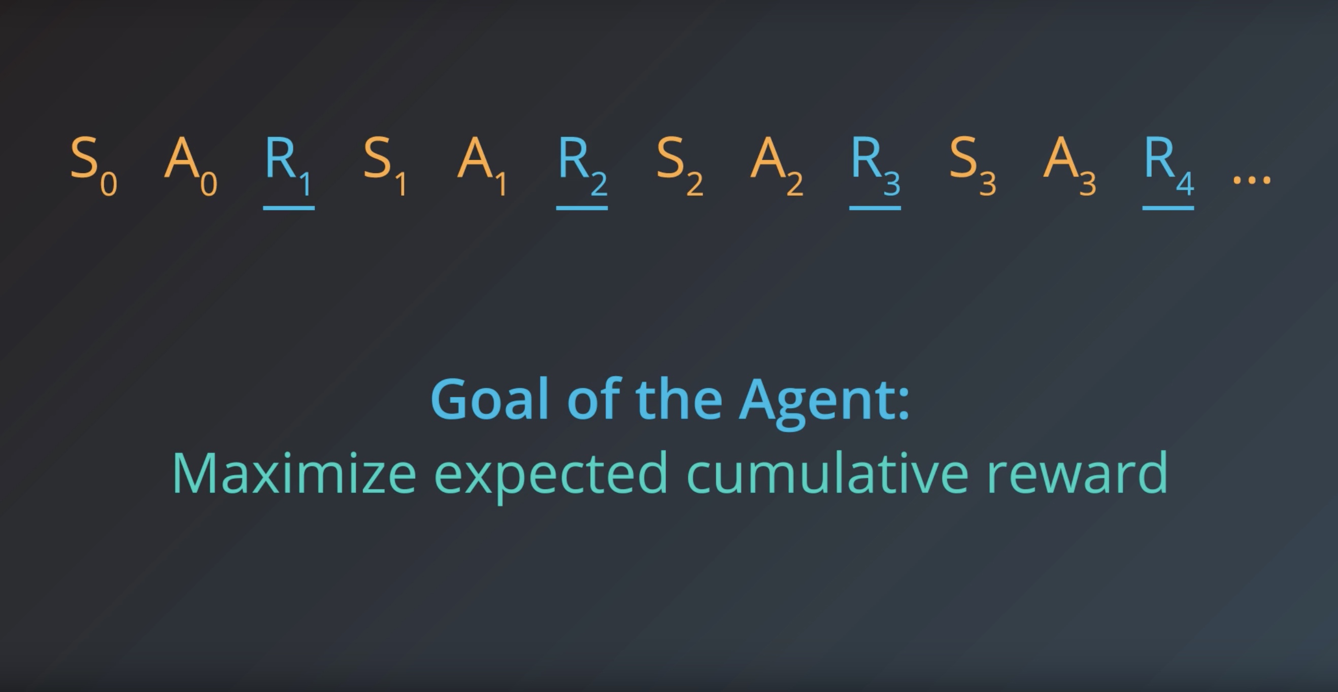
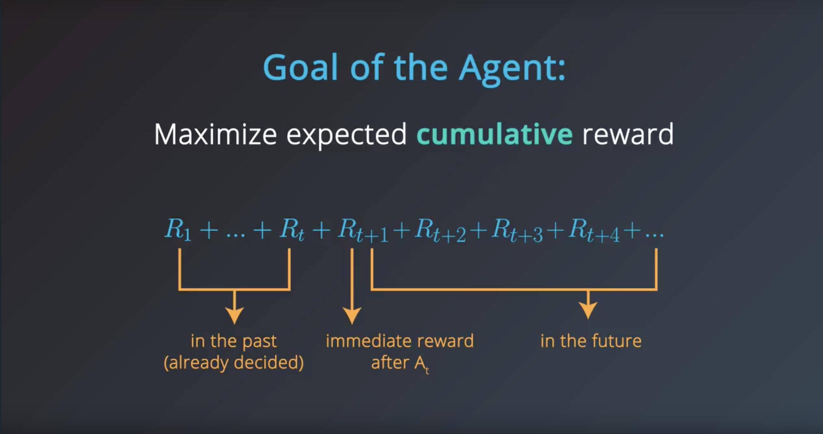
Goal of the Agent = Maximize expected cumulative reward

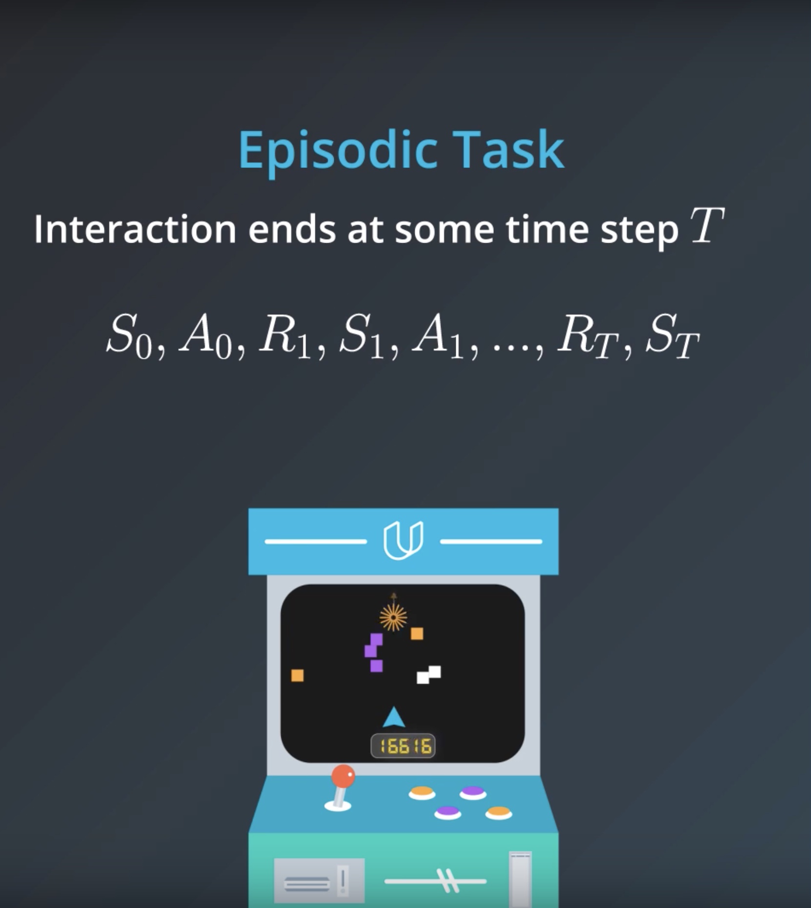
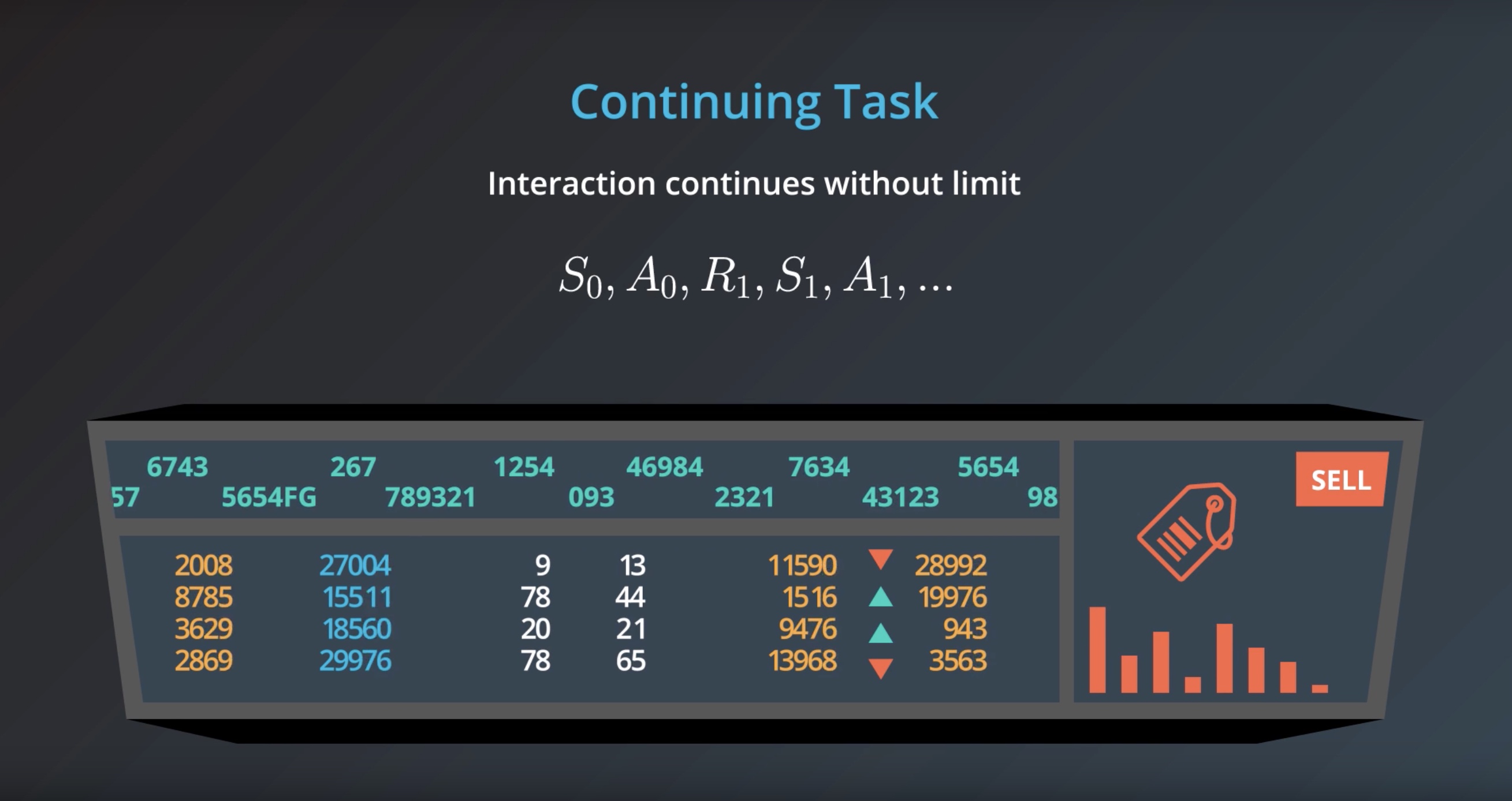
1-1-2 : Episodic vs. Continuing Tasks

from IPython.display import Image
Image(filename='./images/1-1-2-1_episodic_task.jpeg')

from IPython.display import Image
Image(filename='./images/1-1-2-2_continuing_task.jpeg')

1-1-3 : The Reward Hypothesis

from IPython.display import Image
Image(filename='./images/1-1-3-1_agent_have_a_goal.jpeg')

from IPython.display import Image
Image(filename='./images/1-1-3-2_the_reward_hypothesis.jpeg')

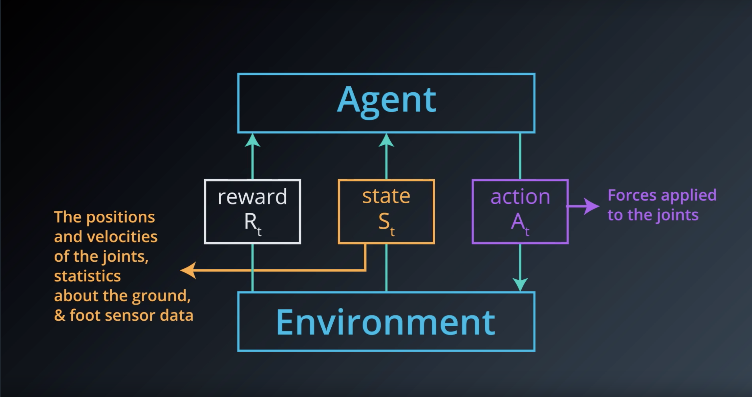
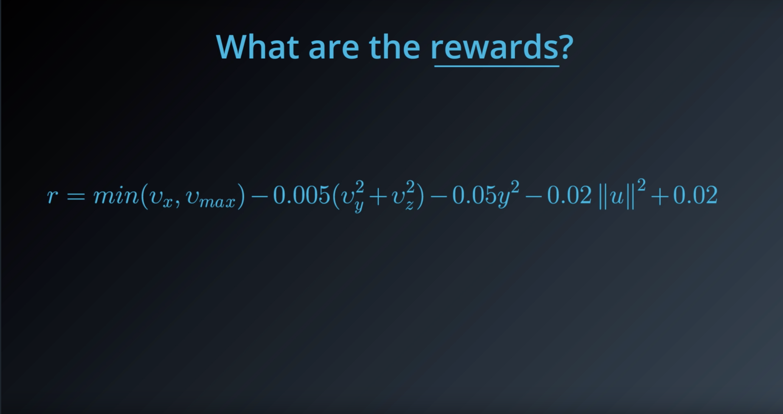
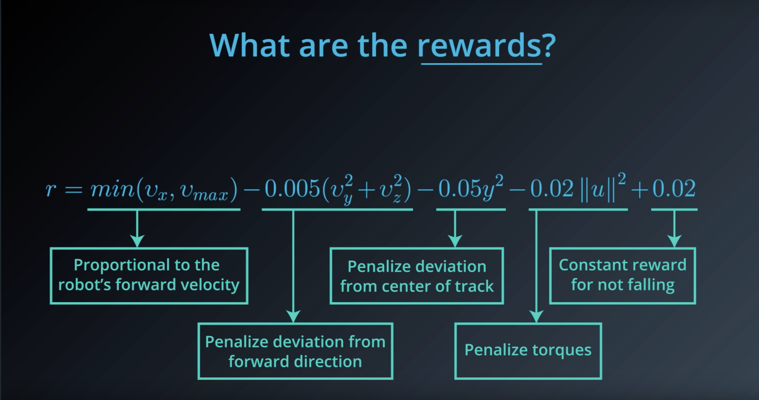
1-1-4 : Goals and Rewards

from IPython.display import Image
Image(filename='./images/1-1-4-1_google_deepmind_robot_learning_to_walk_in_simulateed_env_planar.gif')

<IPython.core.display.Image object>

from IPython.display import Image
Image(filename='./images/1-1-4-2_google_deepmind_robot_learning_to_walk_in_simulateed_env_ant.gif')

<IPython.core.display.Image object>

from IPython.display import Image
Image(filename='./images/1-1-4-3_google_deepmind_robot_learning_to_walk_in_simulateed_env_humanoid.gif')

<IPython.core.display.Image object>

from IPython.display import HTML
HTML('<iframe width="560" height="315" src="https://www.youtube.com/embed/hx_bgoTF7bs" frameborder="0" allow="accelerometer; autoplay; encrypted-media; gyroscope; picture-in-picture" allowfullscreen></iframe>')

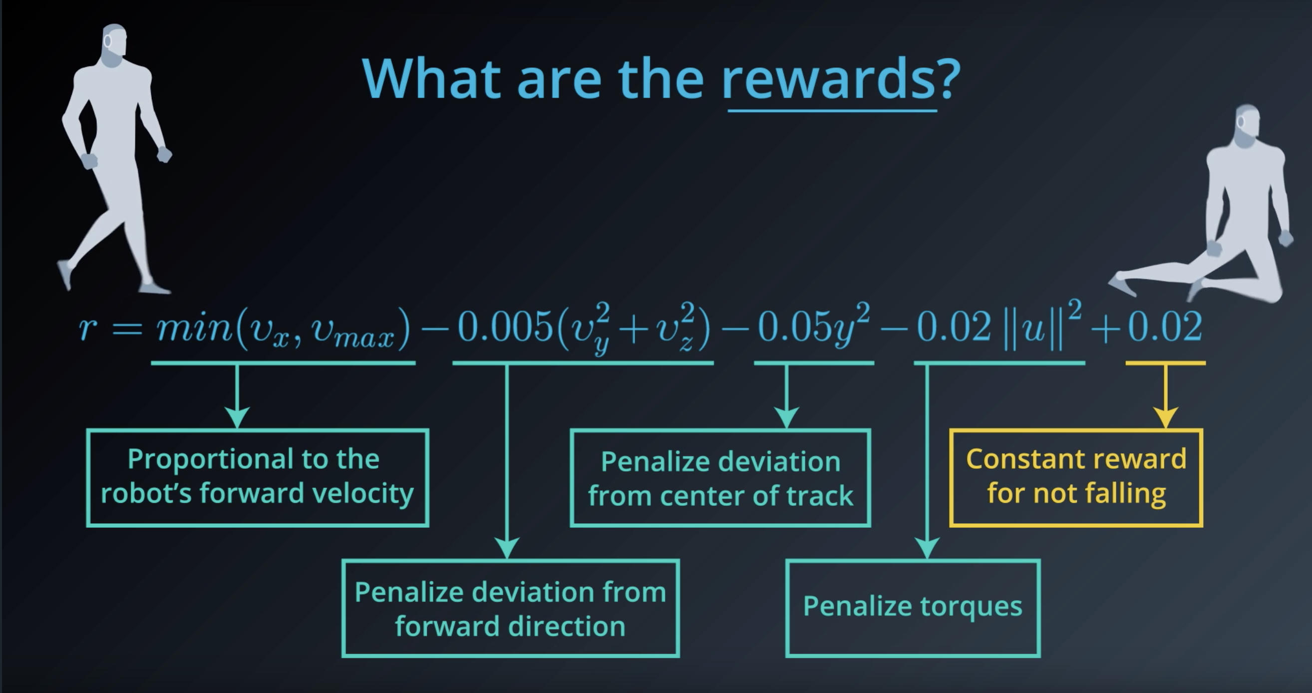
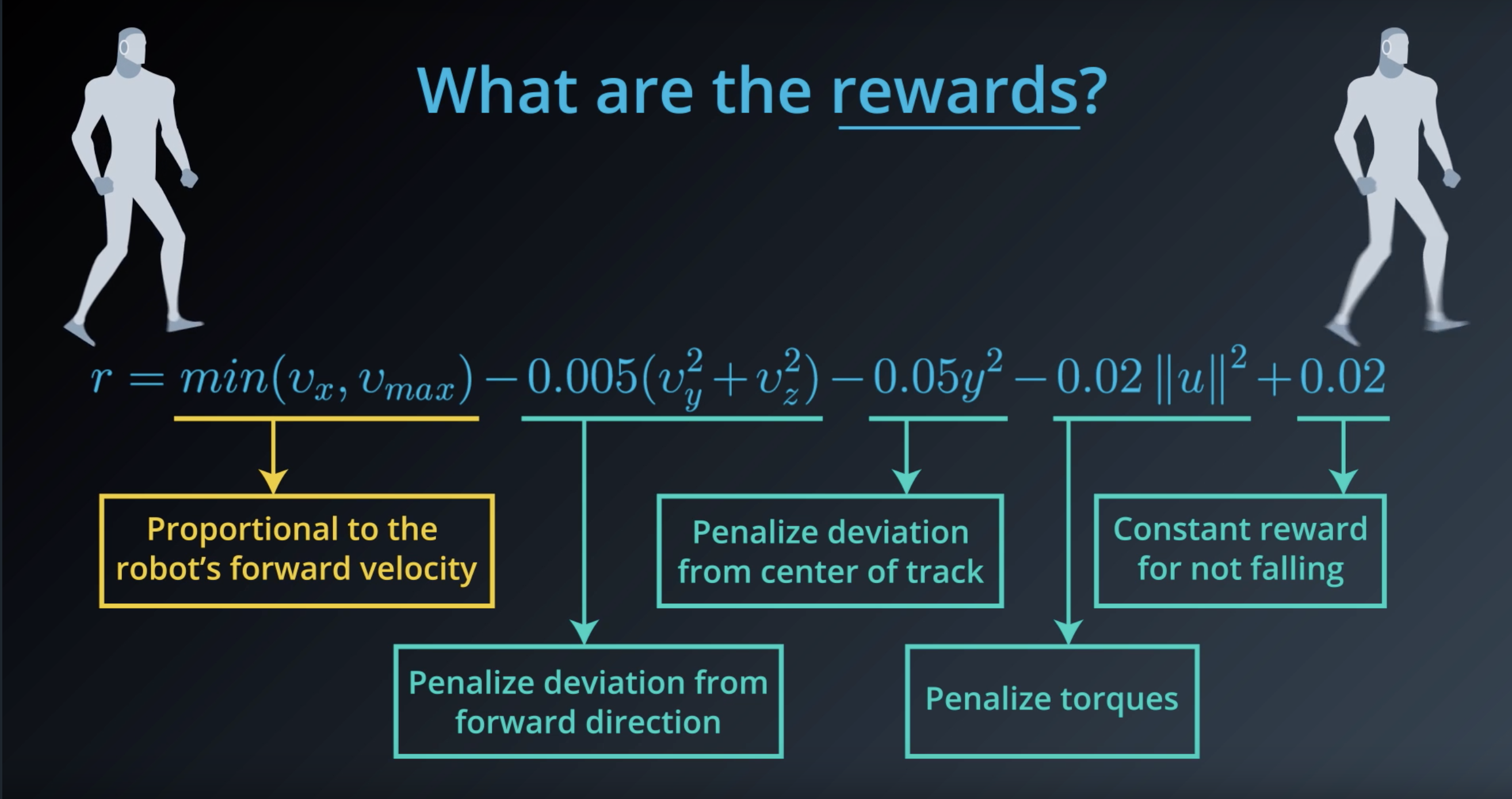
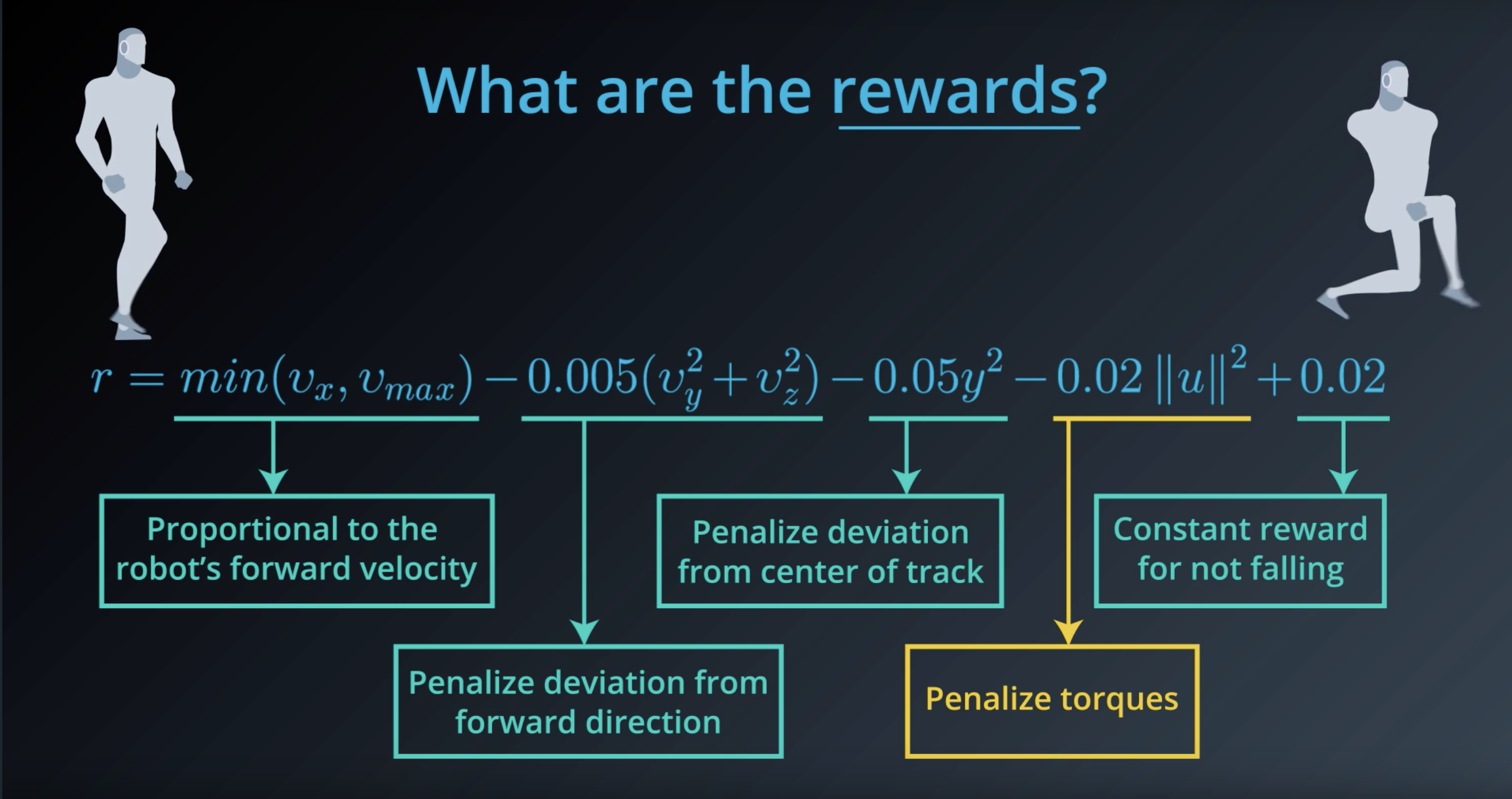
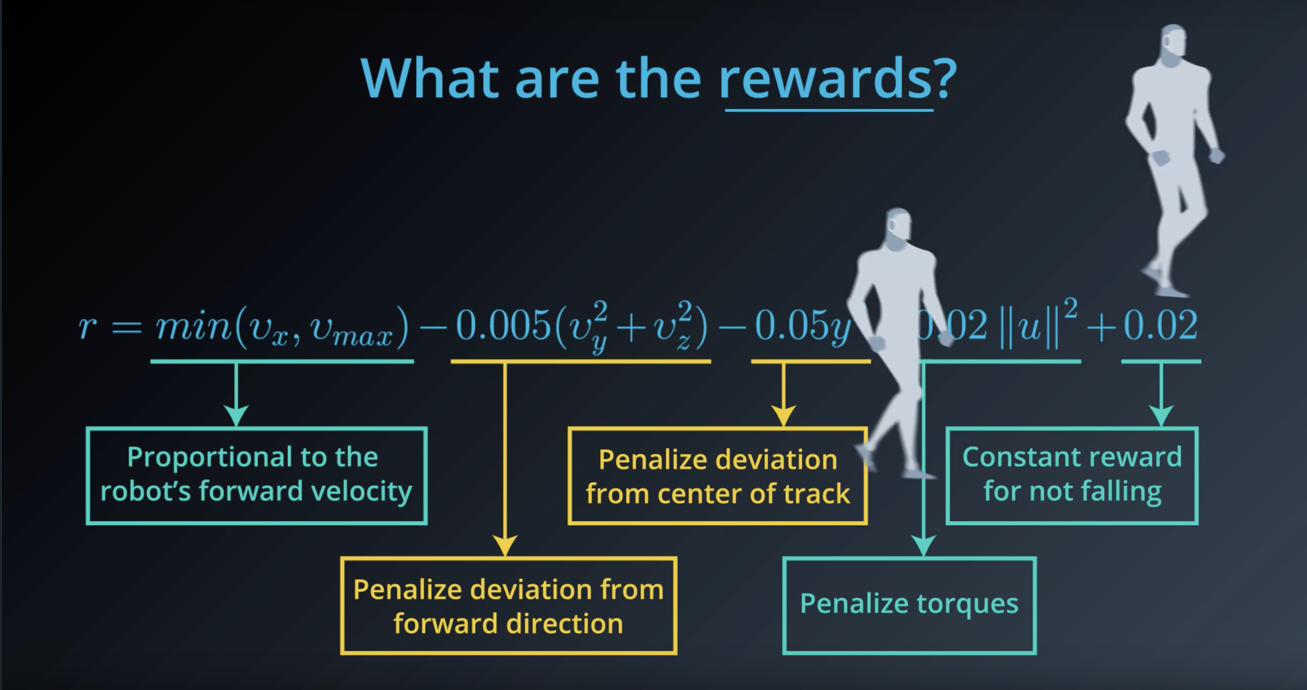
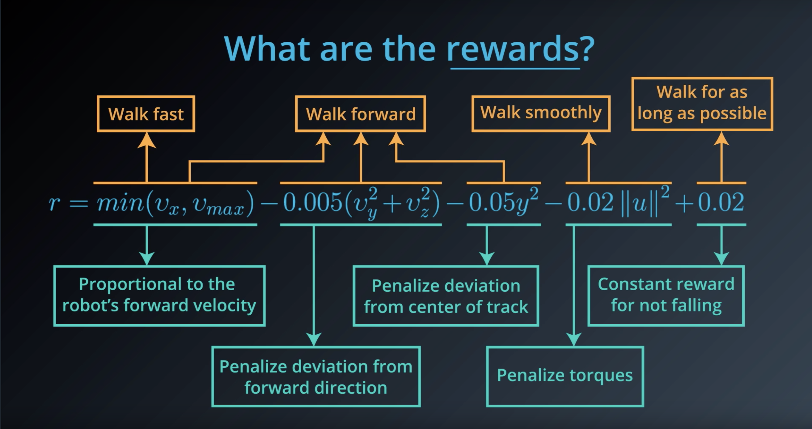
Let’s study the concept of Reward with Google DeepMind 2017 paper “Emergence of Locomotion Behaviours in Rich Environments”

from IPython.display import HTML
HTML('<iframe width="560" height="315" src="https://arxiv.org/pdf/1707.02286.pdf" frameborder="0" allow="accelerometer; autoplay; encrypted-media; gyroscope; picture-in-picture" allowfullscreen></iframe>')

from IPython.display import Image
Image(filename='./images/1-1-4-4_what_are_the_actions.png')

from IPython.display import Image
Image(filename='./images/1-1-4-5_what_are_the_actions_example.png')

from IPython.display import Image
Image(filename='./images/1-1-4-6_what_are_the_states.png')

from IPython.display import Image
Image(filename='./images/1-1-4-7_what_are_the_states_example.png')

from IPython.display import Image
Image(filename='./images/1-1-4-8_what_are_the_rewards.png')

from IPython.display import Image
Image(filename='./images/1-1-4-9_what_are_the_rewards_explain_each.png')

from IPython.display import Image
Image(filename='./images/1-1-4-10_constant_reward_for_not_falling.png')

from IPython.display import Image
Image(filename='./images/1-1-4-11_proportional_to_the_robots_forward_velocity.png')

from IPython.display import Image
Image(filename='./images/1-1-4-12_penalize_torques.png')

from IPython.display import Image
Image(filename='./images/1-1-4-13_penalize_deviation_from_forward_direction_and_from_center_of_track.png')

from IPython.display import Image
Image(filename='./images/1-1-4-14_reward_feedback_to_agent_behavior.png')

from IPython.display import Image
Image(filename='./images/1-1-4-15_reward_from_video_shooting_game.png')

from IPython.display import Image
Image(filename='./images/1-1-4-16_reward_from_backgammon_board-game.png')

1-1-5 : Cumulative Reward

from IPython.display import Image
Image(filename='./images/1-1-5-1_goal_of_the_agent_maximize_expected_cumulative_reward.png')

from IPython.display import Image
Image(filename='./images/1-1-5-2_definition_of_Gt.png')

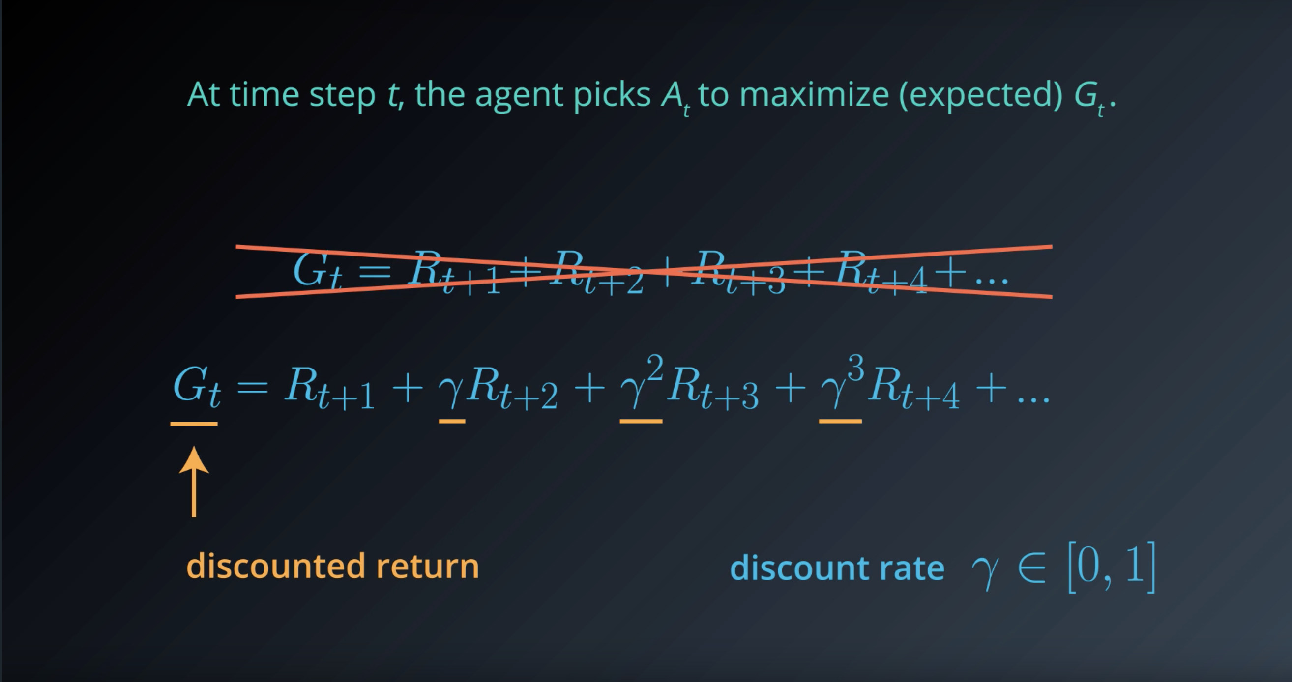
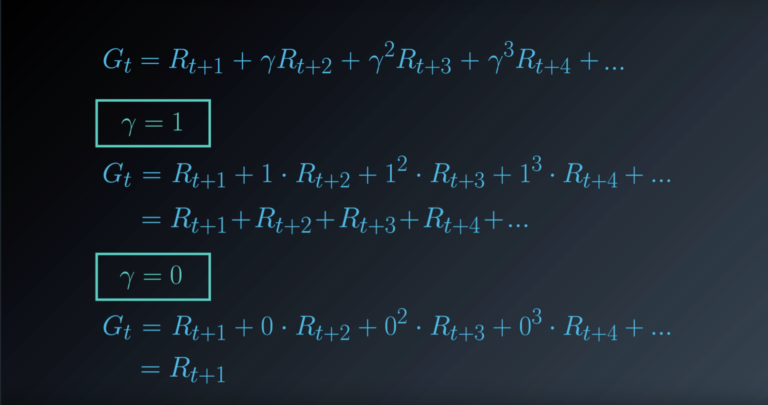
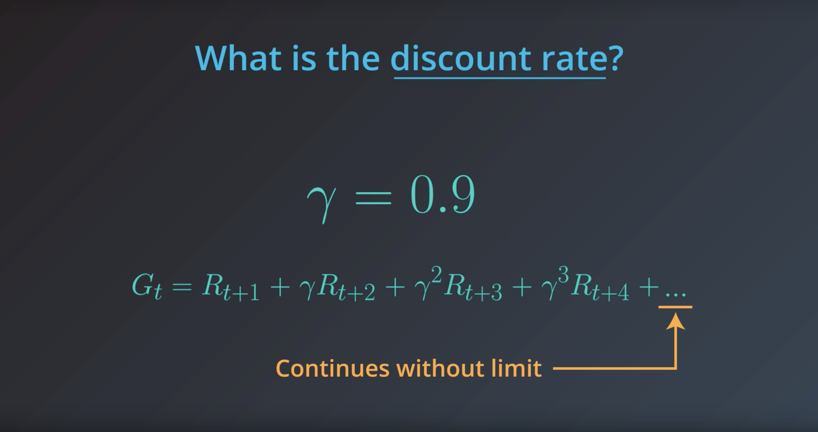
1-1-6 : Discounted Return

from IPython.display import Image
Image(filename='./images/1-1-6-1_discounted_rerurn_gamma_is_0.9.png')

from IPython.display import Image
Image(filename='./images/1-1-6-2_discounted_rerurn_gamma.png')

from IPython.display import Image
Image(filename='./images/1-1-6-3_discounted_rerurn_gamma_is_1_or_0.png')

Quiz : Pole-Balancing

In this classic reinforcement learning task, a cart is positioned on a frictionless track, and a pole is attached to the top of the cart. The objective is to keep the pole from falling over by moving the cart either left or right, and without falling off the track.

In the OpenAI Gym implementation, the agent applies a force of +1 or -1 to the cart at every time step. It is formulated as an episodic task, where the episode ends when (1) the pole falls more than 20.9 degrees from vertical, (2) the cart moves more than 2.4 units from the center of the track, or (3) when more than 200 time steps have elapsed. The agent receives a reward of +1 for every time step, including the final step of the episode. You can read more about this environment in OpenAI’s github. This task also appears in Example 3.4 of the textbook.

from IPython.display import Image
Image(filename='./images/1-1-6-4_cartpole_image.gif')

<IPython.core.display.Image object>

QUESTION 1 OF 3

Recall that the agent receives a reward of +1 for every time step, including the final step of the episode. Which discount rates would encourage the agent to keep the pole balanced for as long as possible? (Select all that apply.)

1. The discount rate is 1.
2. The discount rate is 0.9.
3. The discount rate is 0.5.

QUESTION 2 OF 3

Say that the reward signal is amended to only give reward to the agent at the end of an episode. So, the reward is 0 for every time step, with the exception of the final time step. When the episode terminates, the agent receives a reward of -1. Which discount rates would encourage the agent to keep the pole balanced for as long as possible? (Select all that apply.)

1. The discount rate is 1.
2. The discount rate is 0.9.
3. The discount rate is 0.5.
4. (None of these discount rates would help the agent, and there is a problem with the reward signal.)

QUESTION 3 OF 3

Say that the reward signal is amended to only give reward to the agent at the end of an episode. So, the reward is 0 for every time step, with the exception of the final time step. When the episode terminates, the agent receives a reward of +1. Which discount rates would encourage the agent to keep the pole balanced for as long as possible? (Select all that apply.)

1. The discount rate is 1.
2. The discount rate is 0.9.
3. The discount rate is 0.5.
4. (None of these discount rates would help the agent, and there is a problem with the reward signal.)

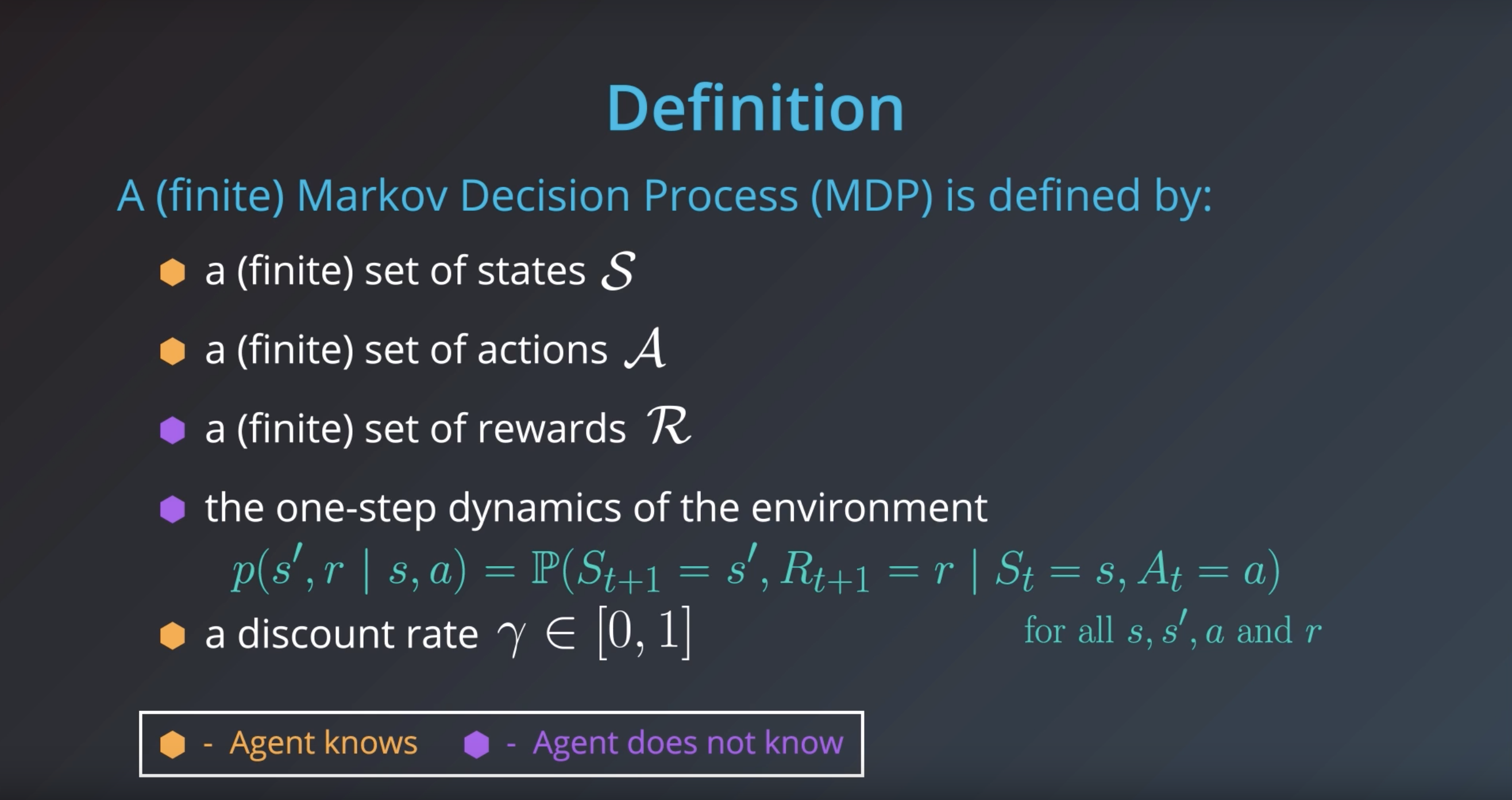
1-1-7 : MDPs

• We’ll learn all about how to rigorously define a reinforcement learning problem as a Markov Decision Process (MDP).
• We will work with the example of recycling robot from the Sutton textbook(Sutton_RL_bookdraft2018.pdf Page 52). (The recycling robot example was inspired by the can-collecting robot built by Jonathan Connell (1989))

from IPython.display import Image
Image(filename='./images/1-1-7-1_consider_a_robot_designed_to_pick_up_empty_soda_cans.png')

from IPython.display import Image
Image(filename='./images/1-1-7-2_robot_keep_search_soda_cans_when_battery_is_high.png')

from IPython.display import Image
Image(filename='./images/1-1-7-3_robot_stop_search_soda_cans_when_battery_is_low.png')

from IPython.display import Image
Image(filename='./images/1-1-7-4_robot_go_to_recharge_when_battery_is_high.png')

from IPython.display import Image
Image(filename='./images/1-1-7-5_robot_recharge_at_the_docking_staton.png')

from IPython.display import Image
Image(filename='./images/1-1-7-6_robot_search_again_after_rechage.png')

from IPython.display import Image
Image(filename='./images/1-1-7-7_robot_have_to_decide_choose_action.png')

from IPython.display import Image
Image(filename='./images/1-1-7-8_robot_focus_on_collectting_as_many_sode_cans_as_possible.png')

from IPython.display import Image
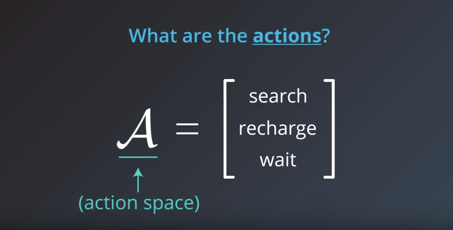
Image(filename='./images/1-1-7-9_recycling_robot_action_space.png')

from IPython.display import Image
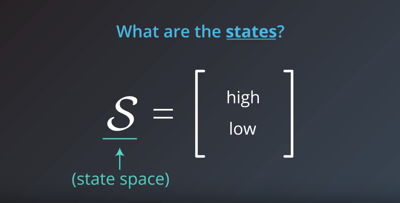
Image(filename='./images/1-1-7-10_recycling_robot_state_space.png')

Notes

• In general, the state space S is the set of all nonterminal states.
• In continuing tasks (like the recycling task), this is equivalent to the set of all states.
• In episodic tasks, we use S+ to refer to the set of all states, including terminal states.
• The action space A is the set of possible actions available to the agent.
• In the event that there are some states where only a subset of the actions are available, we can also use A(s) to refer to the set of actions available in state s∈S.

from IPython.display import Image
Image(filename='./images/1-1-7-11_recycling_robot_state_the_chage_left_on_the_battery.png')

from IPython.display import Image
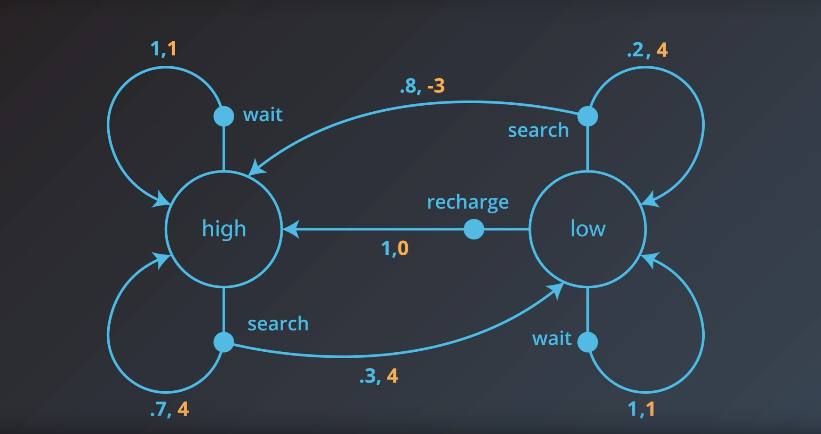
Image(filename='./images/1-1-7-12_recycling_robot_trainsion_and_reward.png')

from IPython.display import Image
Image(filename='./images/1-1-7-13_recycling_robot_trainsion_and_reward_when_bettery_is_high_and_choose_action_search.png')

Quiz: One-Step Dynamics 1

Consider the recycling robot example. In the previous concept, we described one method that the environment could use to decide the state and reward, at any time step.

from IPython.display import Image
Image(filename='./images/1-1-7-15_recycling_robot_quiz_one_step_dynamics.png')

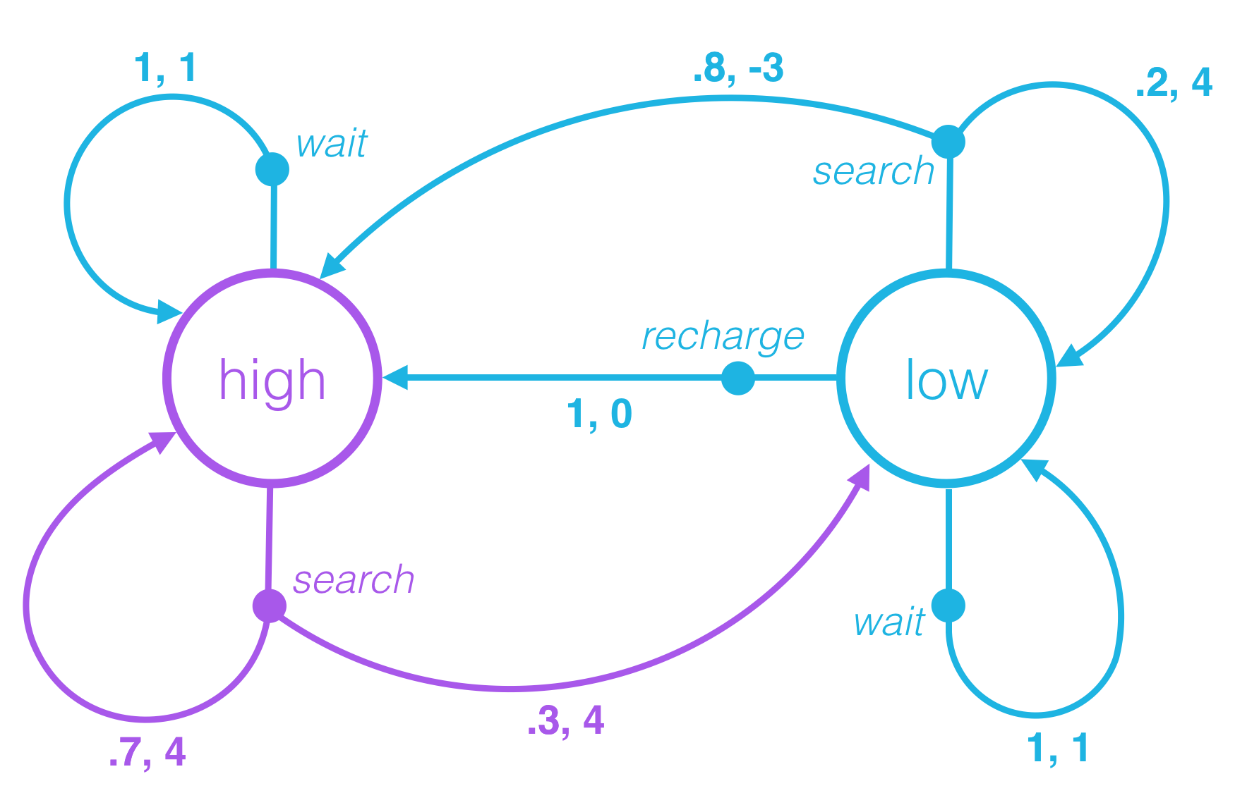
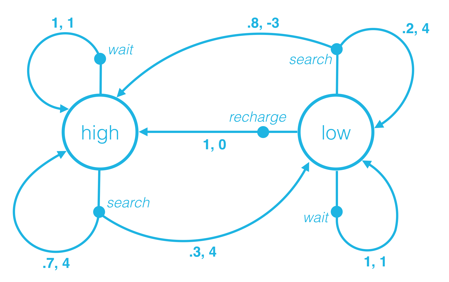
Say at an arbitrary time step t, the state of the robot’s battery is high (St=high). Then, in response, the agent decides to search (At=search). You learned in the previous concept that in this case, the environment responds to the agent by flipping a theoretical coin with 70% probability of landing heads.

If the coin lands heads, the environment decides that the next state is high (St+1=high), and the reward is 4 (Rt+1=4). If the coin lands tails, the environment decides that the next state is low (St+1=low), and the reward is 4 (Rt+1=4). This is depicted in the figure below.

from IPython.display import Image
Image(filename='./images/1-1-7-16_recycling_robot_quiz_one_step_dynamics_when_state_is_hight_action_is_search.png')

In fact, for any state St and action At, it is possible to use the figure to determine exactly how the agent will decide the next state St+1 and reward Rt+1.

QUESTION 1 OF 2

Say the current state is high, and the agent decides to wait. How does the environment decide the next state and reward?

1. With 80% probability, the next state is high, and the reward is -3. With 20% probability, the next state is low, and the reward is 4.
2. The next state is high, and the reward is 1.
3. The next state is low, and the reward is 1.
4. The next state is high, and the reward is 0.

QUESTION 2 OF 2

Say the current state is low, and the agent decides to recharge. How does the environment decide the next state and reward?

1. With 80% probability, the next state is high, and the reward is -3. With 20% probability, the next state is low, and the reward is 4.
2. The next state is high, and the reward is 1.
3. The next state is low, and the reward is 1.
4. The next state is high, and the reward is 0.

Quiz: One-Step Dynamics 2

It will prove convenient to represent the environment’s dynamics using mathematical notation. In this concept, we will introduce this notation (which can be used for any reinforcement learning task) and use the recycling robot as an example.

from IPython.display import Image
Image(filename='./images/1-1-7-15_recycling_robot_quiz_one_step_dynamics.png')

At an arbitrary time step t, the agent-environment interaction has evolved as a sequence of states, actions, and rewards

(S0,A0,R1,S1,A1,…,Rt−1,St−1,At−1,Rt,St,At).

When the environment responds to the agent at time step t+1, it considers only the state and action at the previous time step (St,At).

In particular, it does not care what state was presented to the agent more than one step prior. (In other words, the environment does not consider any of {S0,…,St−1}.)

And, it does not look at the actions that the agent took prior to the last one. (In other words, the environment does not consider any of {A0,…,At−1}.)

Furthermore, how well the agent is doing, or how much reward it is collecting, has no effect on how the environment chooses to respond to the agent. (In other words, the environment does not consider any of {R0,…,Rt}.)

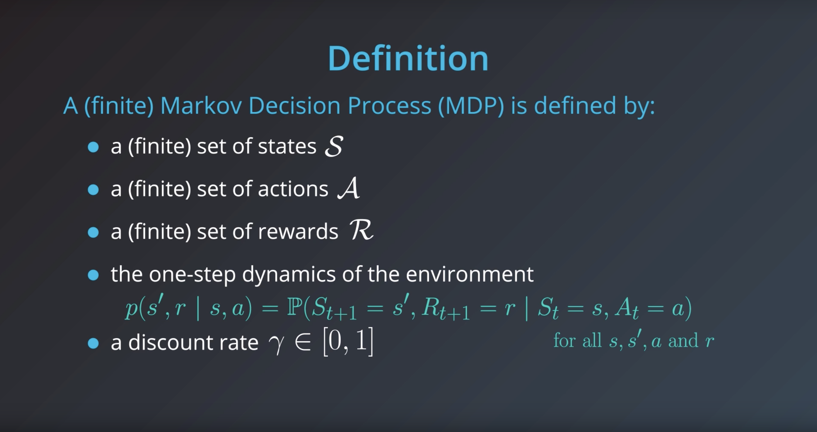
Because of this, we can completely define how the environment decides the state and reward by specifying

p(s′,r∣s,a)≐P(St+1=s′,Rt+1=r∣St=s,At=a)

for each possible s′,r,s,and a. These conditional probabilities are said to specify the one-step dynamics of the environment.

from IPython.display import Image
Image(filename='./images/1-1-7-16_recycling_robot_quiz_one_step_dynamics_when_state_is_hight_action_is_search.png')

An Example

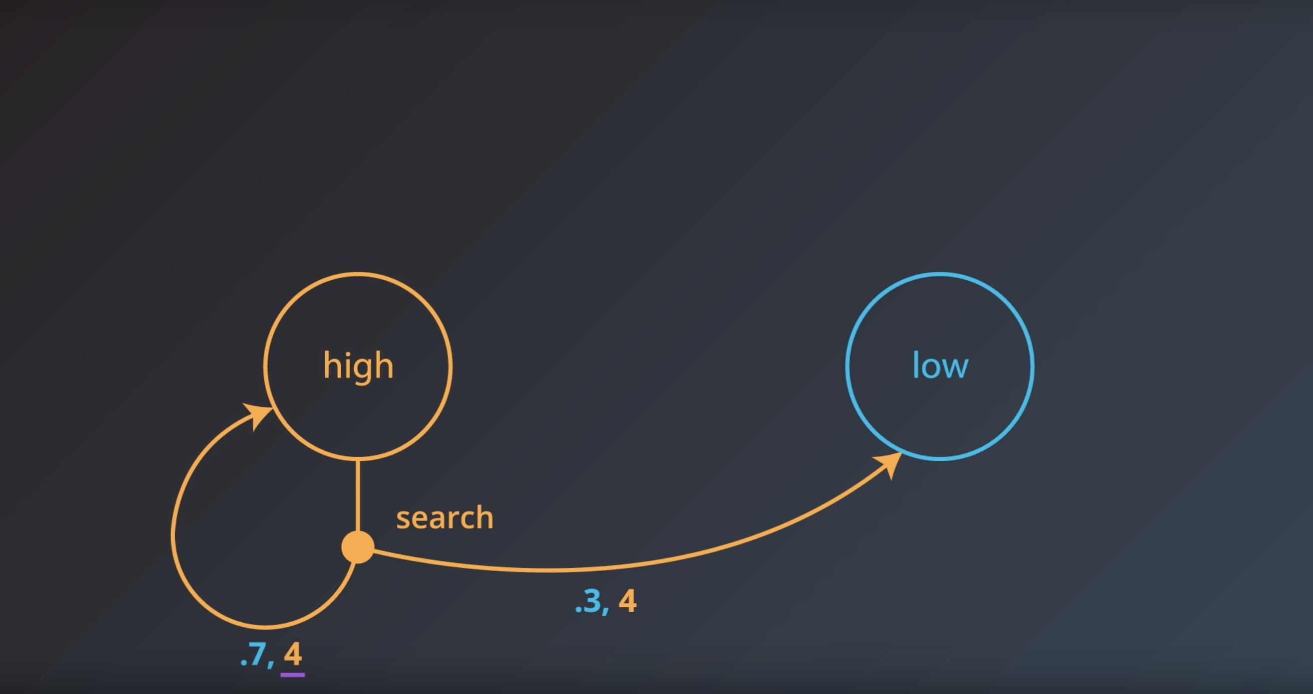
Let’s return to the case that St=high, and At =search.

Then, when the environment responds to the agent at the next time step,

with 70% probability, the next state is high and the reward is 4. In other words,

p(high,4∣high,search)=P(St+1=high,Rt+1=4∣St=high,At=search)=0.7.

with 30% probability, the next state is low and the reward is 4. In other words,

p(low,4∣high,search)=P(St+1=low,Rt+1=4∣St=high,At=search)=0.3.

QUESTION 1

What is p(high,−3∣low,search)? Calcurate the correct numerical value.

QUESTION 2

What is p(high,0∣low,recharge)? Calcurate the correct numerical value.

QUESTION 3

Consider the following probabilities:

• (1) p(low,1∣low,search)
• (2) p(high,0∣low,recharge)
• (3) p(high,1∣low,wait)
• (4) p(high,1∣high,wait)
• (5) p(high,1∣high,search)

Which of the above probabilities is equal to 0? (Select all that apply.)

QUESTION 4

Consider the following probabilities:

• (1) p(low,1∣low,search)
• (2) p(high,0∣low,recharge)
• (3) p(high,1∣low,wait)
• (4) p(high,1∣high,wait)
• (5) p(high,1∣high,search)

Which of the above probabilities is equal to 1? (Select all that apply.)

from IPython.display import Image
Image(filename='./images/1-1-7-17_definition_of_finite_mdp.png')

from IPython.display import Image
Image(filename='./images/1-1-7-18_definition_of_finite_mdp_what_is_the_discount_rate.png')

from IPython.display import Image
Image(filename='./images/1-1-7-19_definition_of_finite_mdp_what_agent_know_and_what_agent_do_not_know.png')

1-1-8 : Finite MDPs

from IPython.display import Image
Image(filename='./images/1-1-8-1_finite_mdp_openai_gym_environment.png')

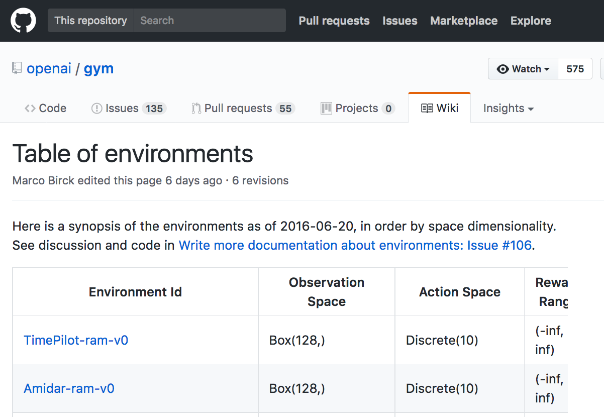
Please use this link to peruse the available environments in OpenAI Gym.

The environments are indexed by Environment Id, and each environment has corresponding Observation Space, Action Space, Reward Range, tStepL, Trials, and rThresh.

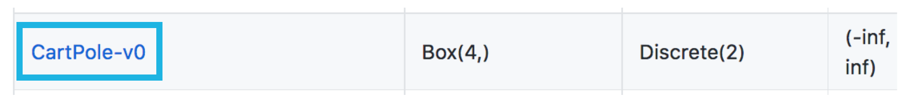
CartPole-v0

Find the line in the table that corresponds to the CartPole-v0 environment. Take note of the corresponding Observation Space (Box(4,)) and Action Space (Discrete(2)).

Every environment comes with first-class Space objects that describe the valid actions and observations.

• The Discrete space allows a fixed range of non-negative numbers.
• The Box space represents an n-dimensional box, so valid actions or observations will be an array of n numbers.

from IPython.display import Image
Image(filename='./images/1-1-8-2_finite_mdp_openai_gym_cartpole.png')

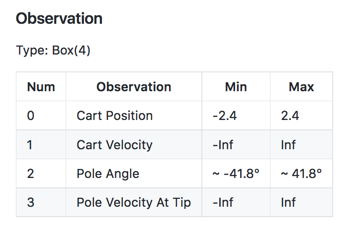
Observation Space

The observation space for the CartPole-v0 environment has type Box(4,). Thus, the observation (or state) at each time point is an array of 4 numbers. You can look up what each of these numbers represents in this document. After opening the page, scroll down to the description of the observation space.

Notice the minimum (-Inf) and maximum (Inf) values for both Cart Velocity and the Pole Velocity at Tip.

Since the entry in the array corresponding to each of these indices can be any real number, the state space S+ is infinite!

from IPython.display import Image
Image(filename='./images/1-1-8-3_finite_mdp_openai_gym_cartpole_observation_space.png')

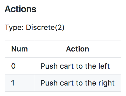
Action Space

The action space for the CartPole-v0 environment has type Discrete(2). Thus, at any time point, there are only two actions available to the agent. You can look up what each of these numbers represents in this document (note that it is the same document you used to look up the observation space!). After opening the page, scroll down to the description of the action space.

In below case, the action space A is a finite set containing only two elements.

from IPython.display import Image
Image(filename='./images/1-1-8-4_finite_mdp_openai_gym_cartpole_action_space.png')

Finite MDPs

Recall from the previous concept that in a finite MDP, the state space S (or S+, in the case of an episodic task) and action space A must both be finite.

Thus, while the CartPole-v0 environment does specify an MDP, it does not specify a finite MDP. In this course, we will first learn how to solve finite MDPs. Then, later in this course, you will learn how to use neural networks to solve much more complex MDPs!

Lesson 1-2: The RL Framework: The Solution

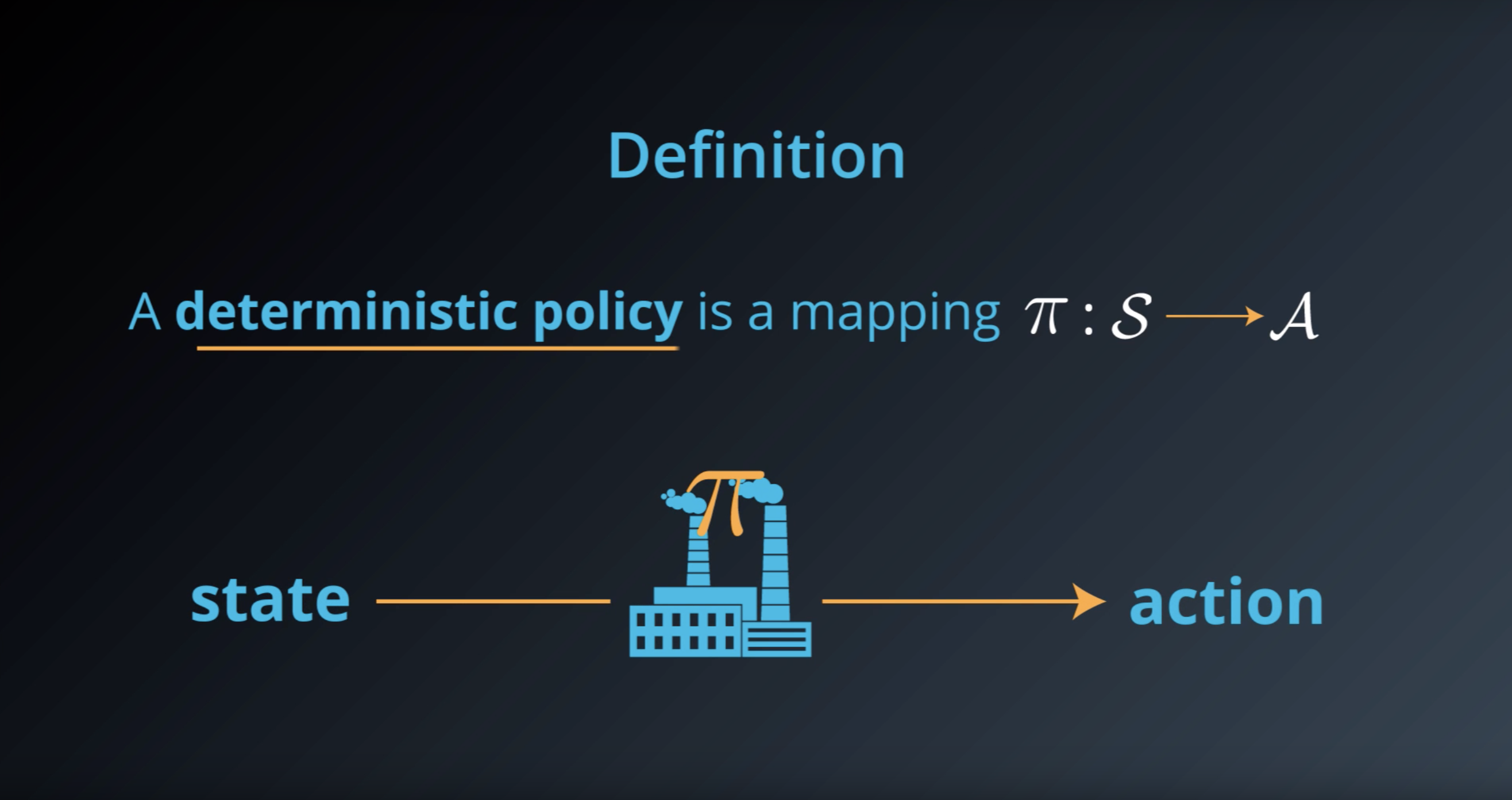
1-2-1 : Policies

from IPython.display import Image
Image(filename='./images/1-2-1-1_definition_of_deterministic_policy.png')

from IPython.display import Image
Image(filename='./images/1-2-1-2_definition_of_stochastic_policy.png')

from IPython.display import Image
Image(filename='./images/1-2-1-3_deterministic_and_stochastic_policy_on_recycling_robot.png')

from IPython.display import Image
Image(filename='./images/1-2-1-4_deterministic_policy_is_stochastic_policy_which_return_1_or_0_posibility.png')

Quiz: Interpret the Policy

A policy determines how an agent chooses an action in response to the current state. In other words, it specifies how the agent responds to situations that the environment has presented.

Consider the recycling robot MDP from the previous lesson.

from IPython.display import Image
Image(filename='./images/1-1-7-15_recycling_robot_quiz_one_step_dynamics.png')

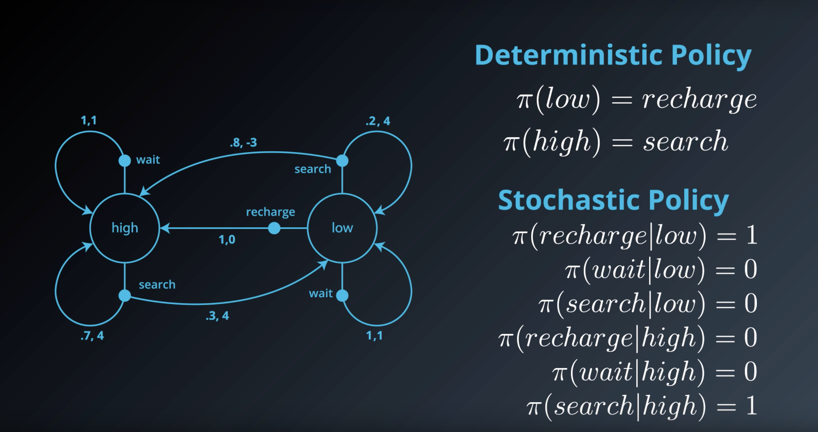
Deterministic Policy: Example

An example deterministic policy π:S→A can be specified as:

• π(low)=recharge
• π(high)=search

In this case,

• if the battery level is low, the agent chooses to recharge the battery.
• if the battery level is high, the agent chooses to search for cans.

QUESTION 1 OF 2

Which of the following statements are true, if the agent follows the policy? (Select all that apply.)

1. If the state is low, the agent chooses action search.
2. If the action is low, the agent chooses state search.
3. The agent will always search for cans at every time step (whether the battery level is low or high).
4. If the state is high, the agent chooses to wait for cans.

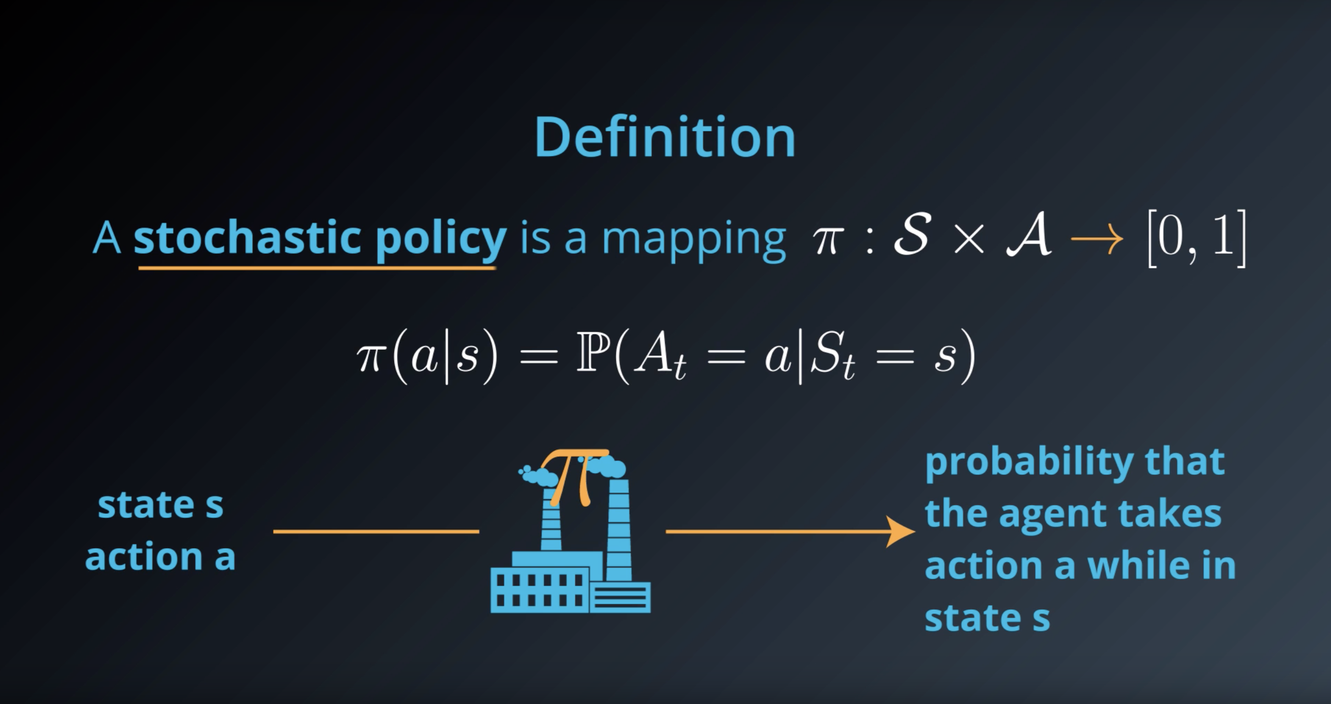
Stochastic Policy: Example

An example stochastic policy π:S×A→[0,1] can be specified as:

• π(recharge∣low)=0.5
• π(wait∣low)=0.4
• π(search∣low)=0.1
• π(search∣high)=0.9
• π(wait∣high)=0.1

In this case,

• if the battery level is low, the agent recharges the battery with 50% probability, waits for cans with 40% probability, and searches for cans with 10% probability.
• if the battery level is high, the agent searches for cans with 90% probability and waits for cans with 10% probability.

QUESTION 2 OF 2

Consider a different stochastic policy π:S×A→[0,1], where:

• π(recharge∣low)=0.3
• π(wait∣low)=0.5
• π(search∣low)=0.2
• π(search∣high)=0.6
• π(wait∣high)=0.4

Which of the following statements are true, if the agent follows the policy? (Select all that apply.)

1. If the battery level is low, the agent will always decide to wait for cans.
2. If the battery level is high, the agent chooses to search for a can with 60% probability, and otherwise waits for a can.
3. If the battery level is low, the agent is most likely to decide to wait for cans.

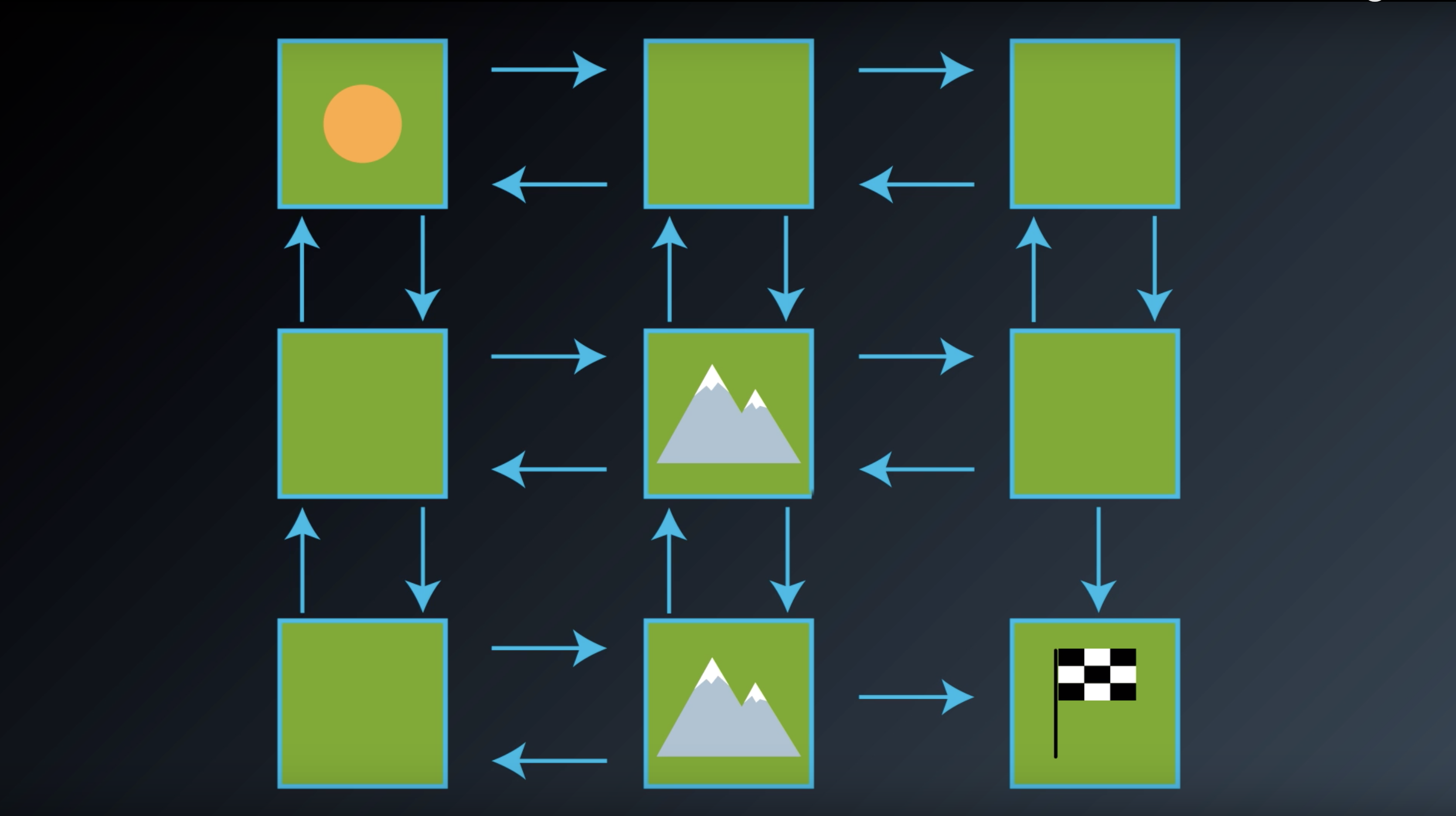
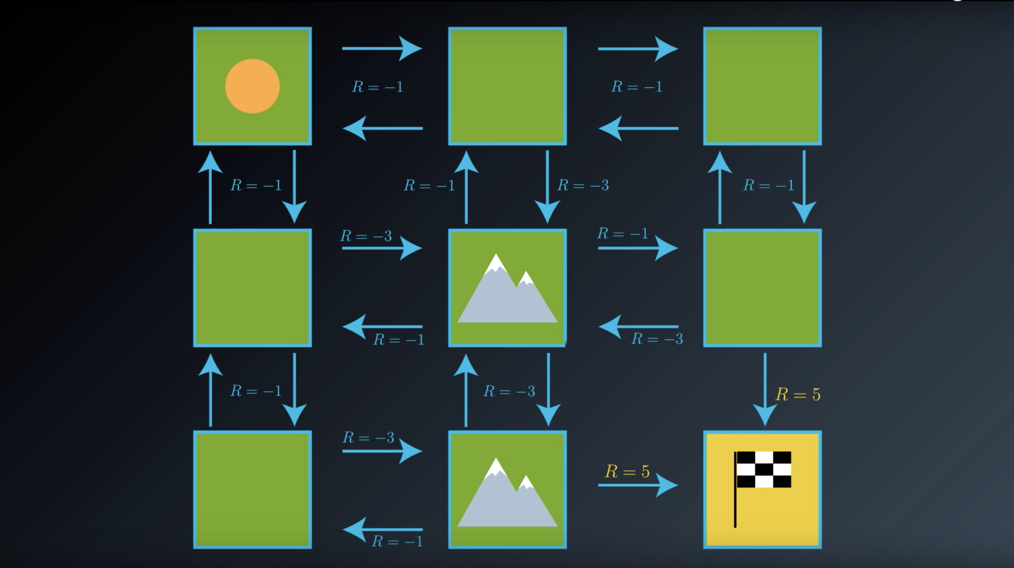
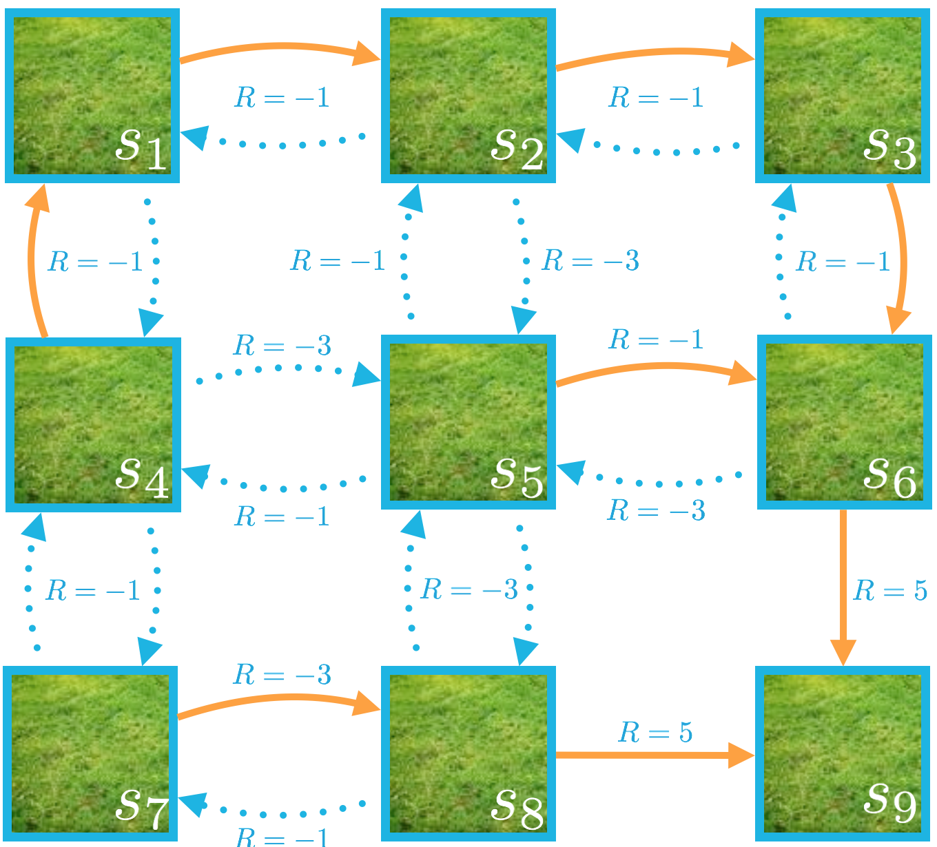
1-2-2 : GridWorld Example

from IPython.display import Image
Image(filename='./images/1-2-2-1_gridworld_with_nine_states_including_two_mountines_states.png')

from IPython.display import Image
Image(filename='./images/1-2-2-2_gridworld_goal_and_action.png')

from IPython.display import Image
Image(filename='./images/1-2-2-3_gridworld_actions_around_terminial_state.png')

from IPython.display import Image
Image(filename='./images/1-2-2-4_gridworld_rewards_with_value_of_minus_1.png')

from IPython.display import Image
Image(filename='./images/1-2-2-5_gridworld_rewards_around_mountain_state_and_terminal_state.png')

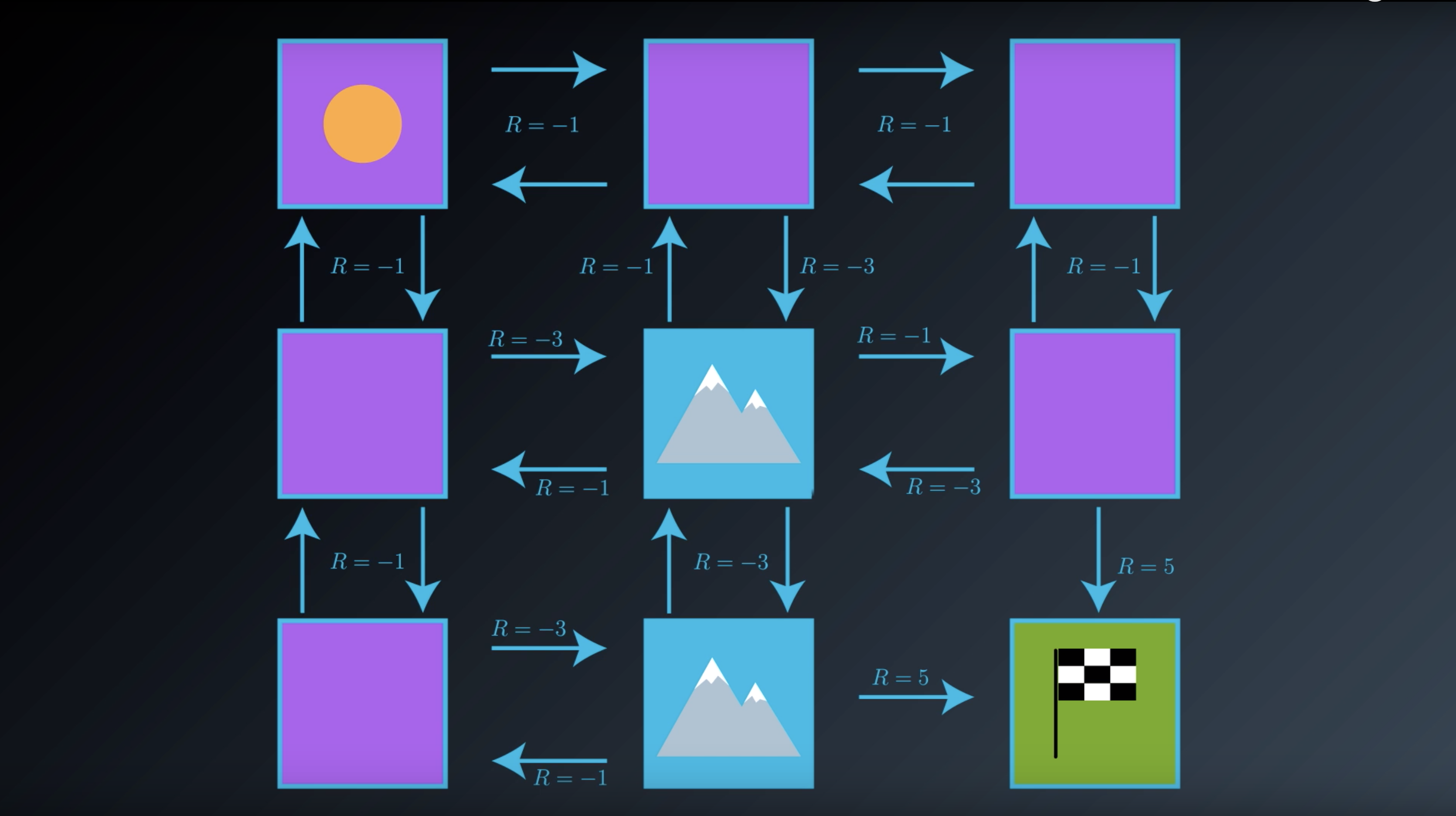
from IPython.display import Image
Image(filename='./images/1-2-2-6_gridworld_rewards_around_terminal_state_with_value_of_plus_5.png')

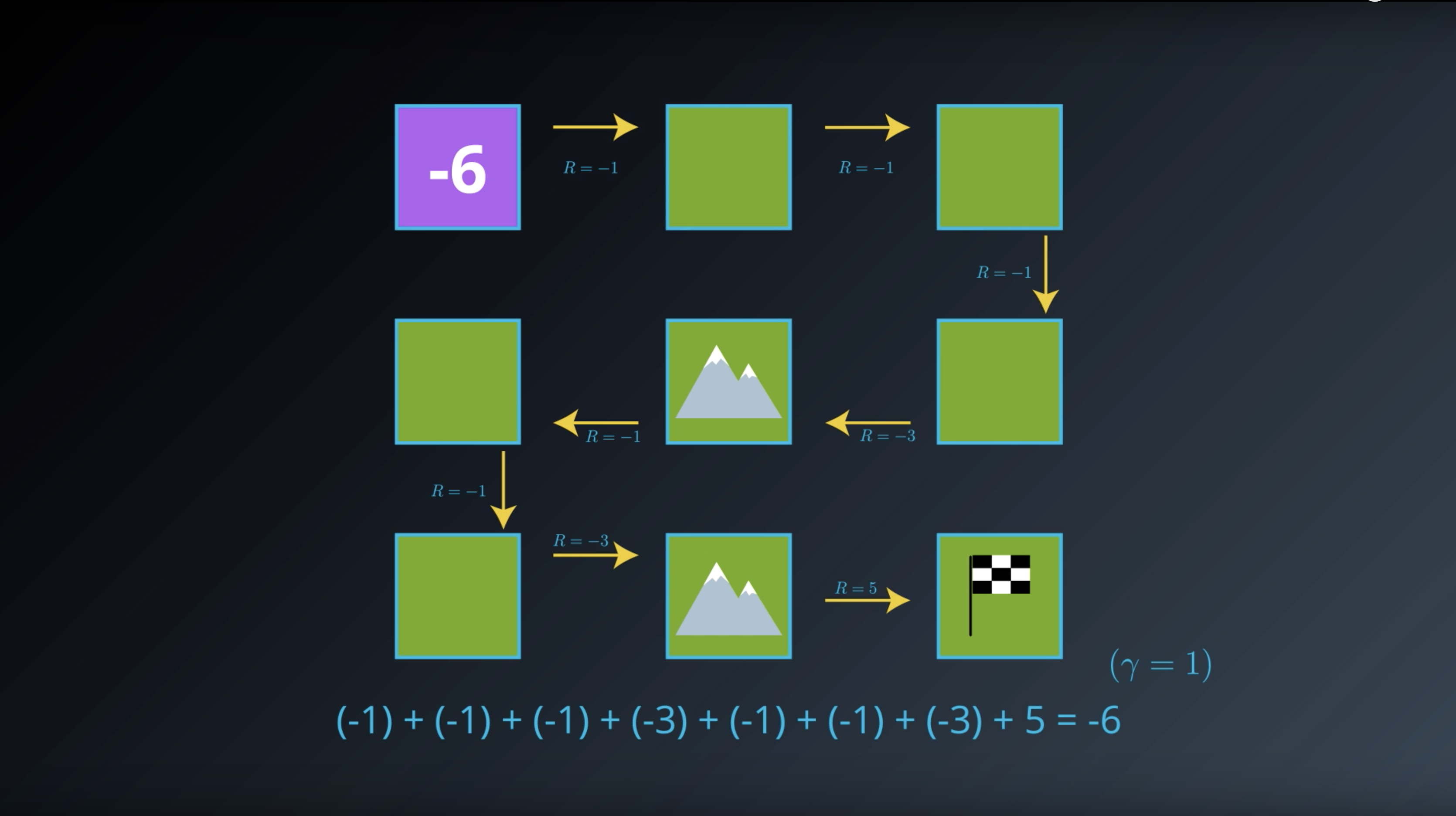
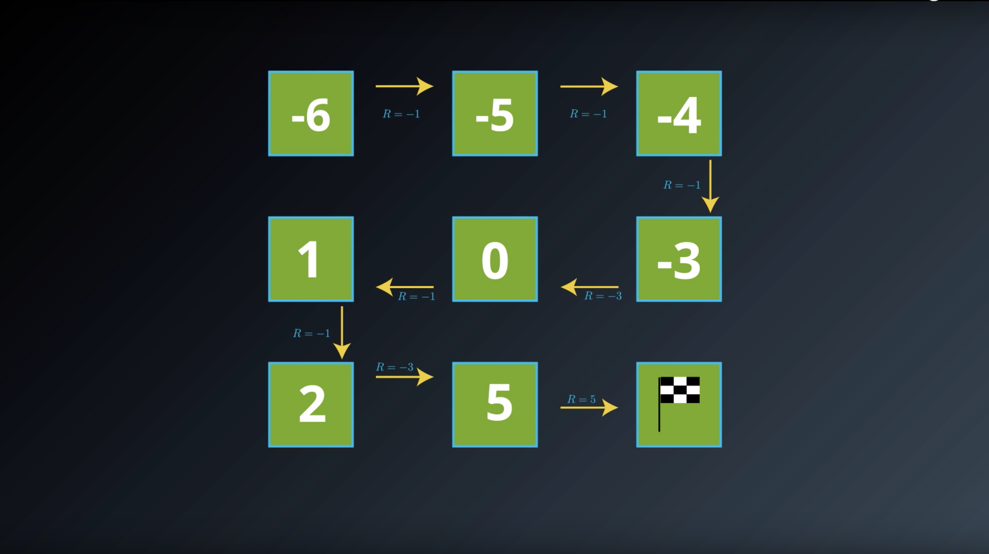
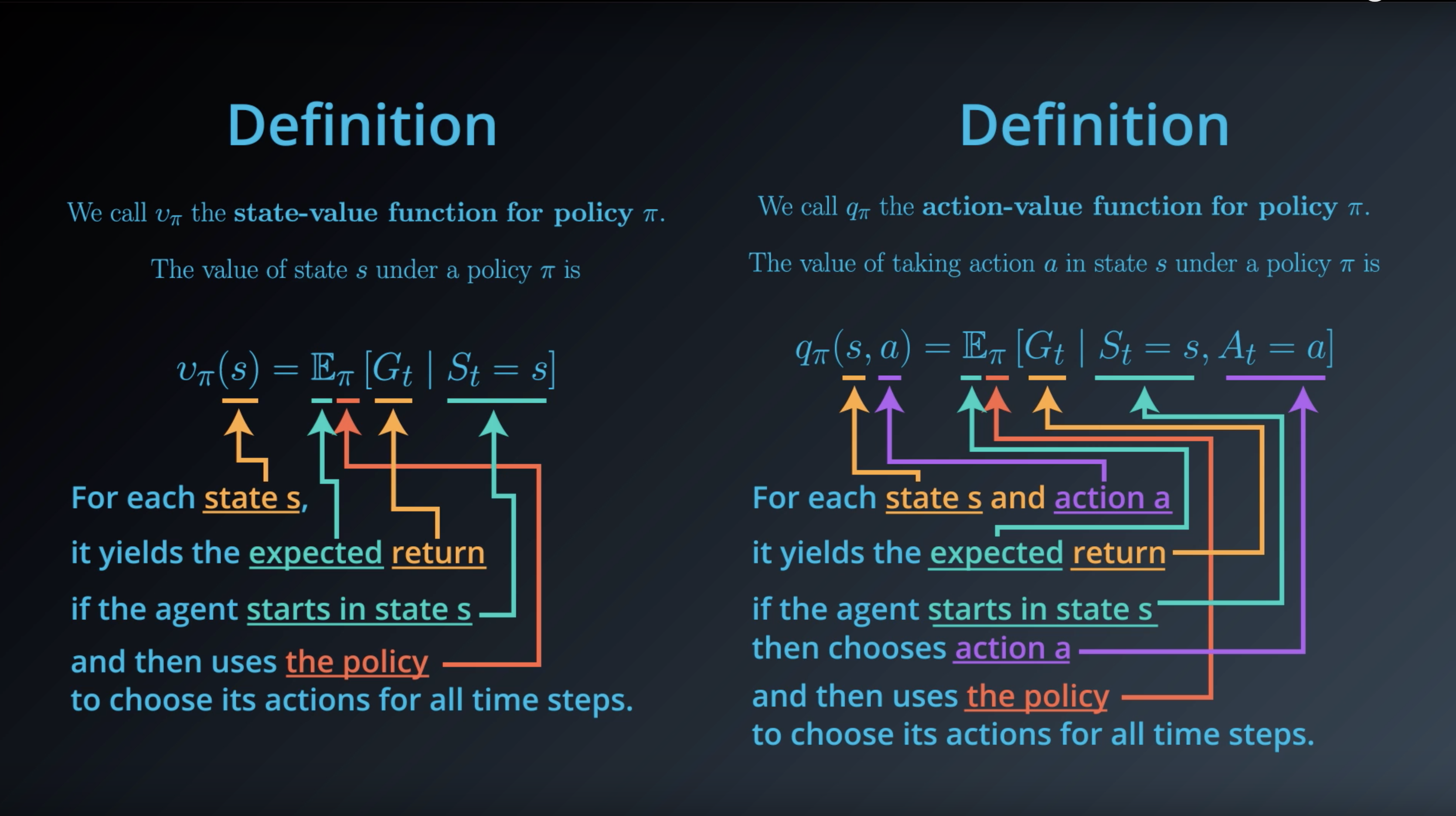
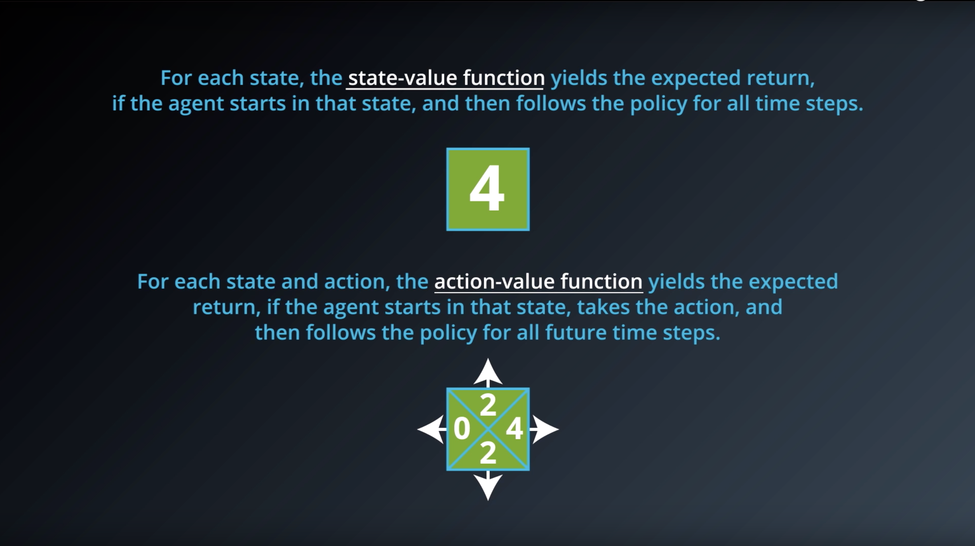
1-2-3. State-Value Functions

from IPython.display import Image
Image(filename='./images/1-2-3-1_state_function_value_of_state1_is_minus_6.png')

from IPython.display import Image
Image(filename='./images/1-2-3-2_state_function_value_of_state1_is_saved_in_transition_table.png')

from IPython.display import Image
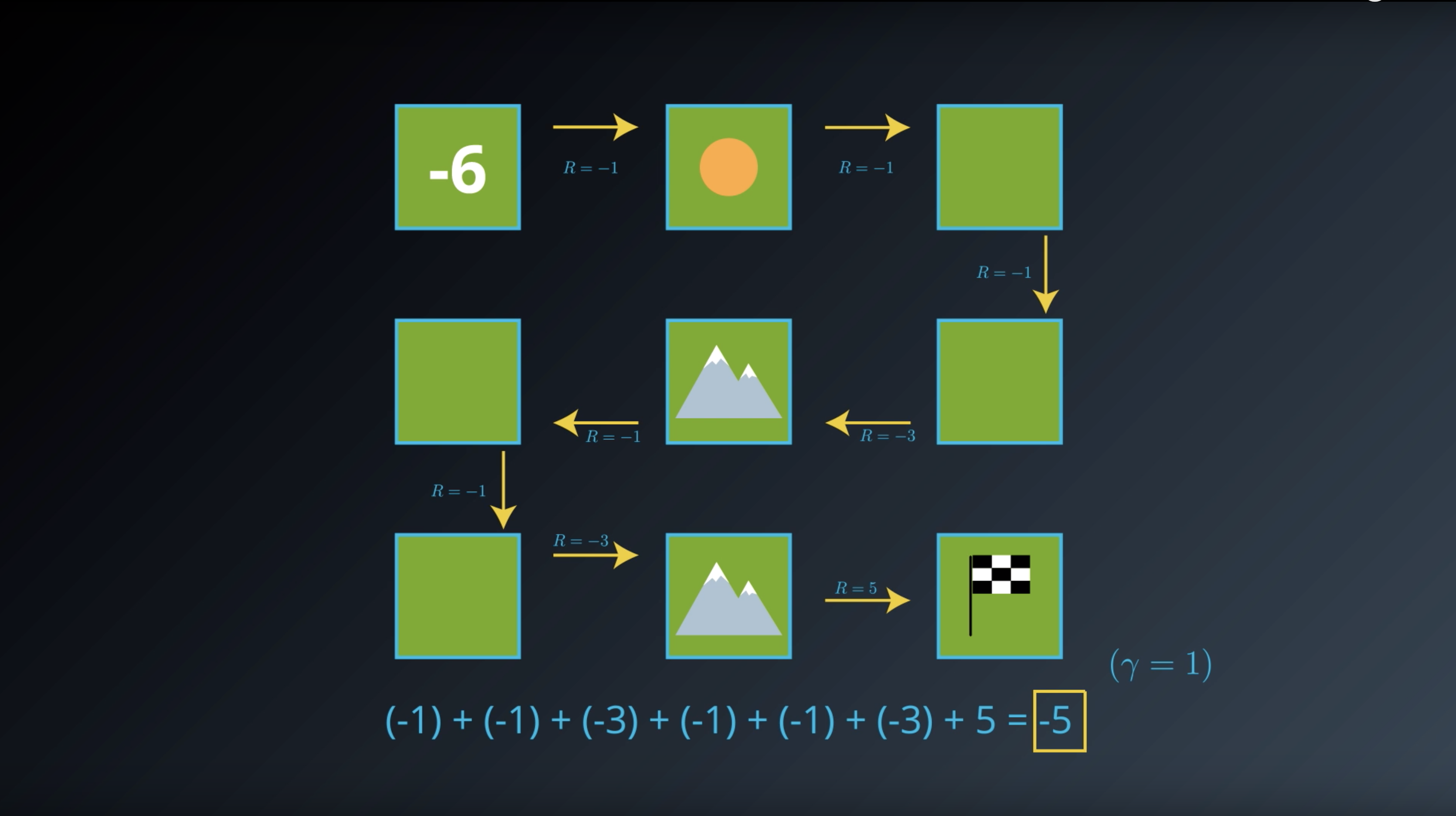
Image(filename='./images/1-2-3-3_state_function_value_of_state2_is_minus_5.png')

from IPython.display import Image
Image(filename='./images/1-2-3-4_state_function_value_of_state2_is_saved_in_transition_table.png')

from IPython.display import Image
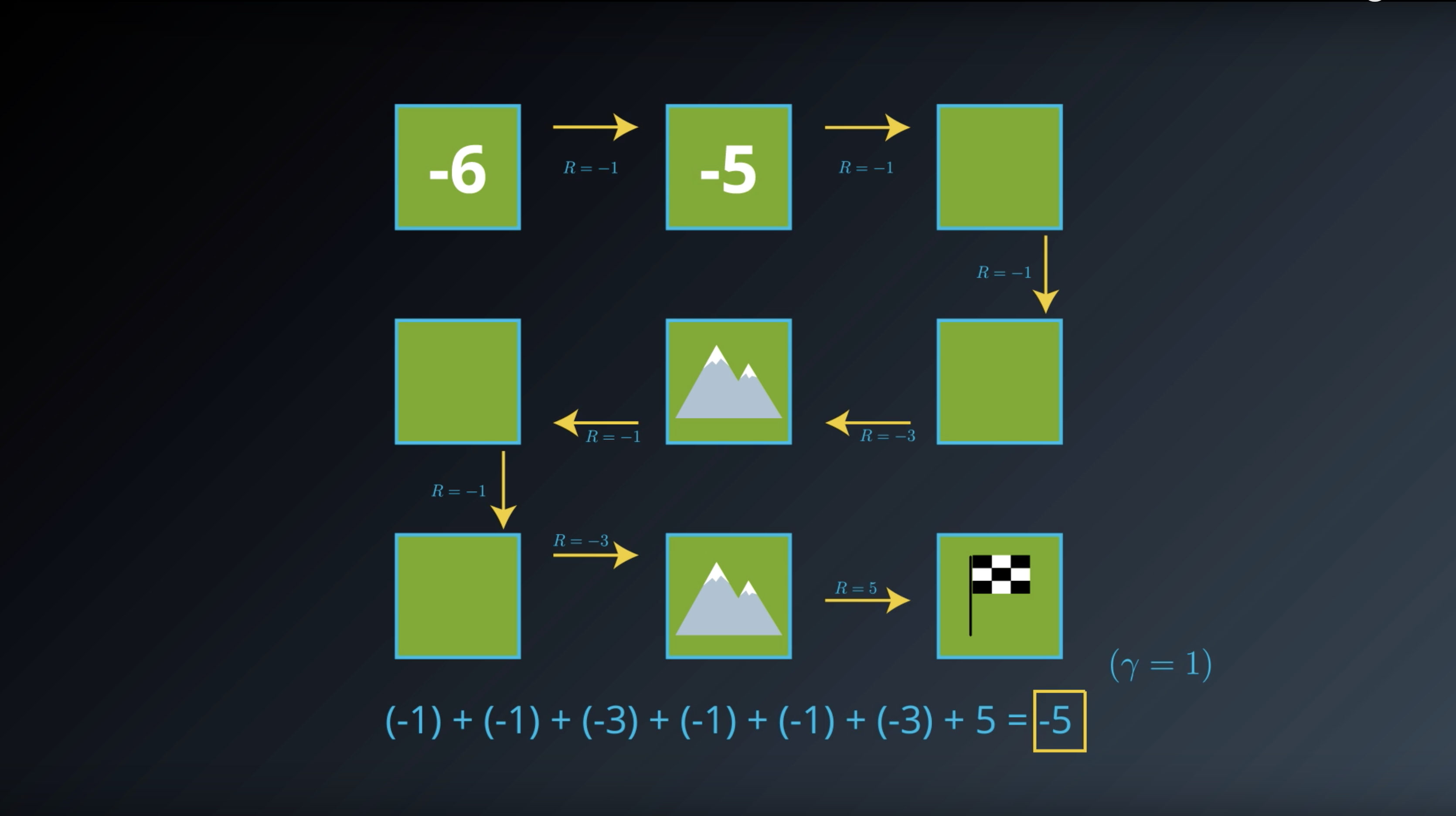
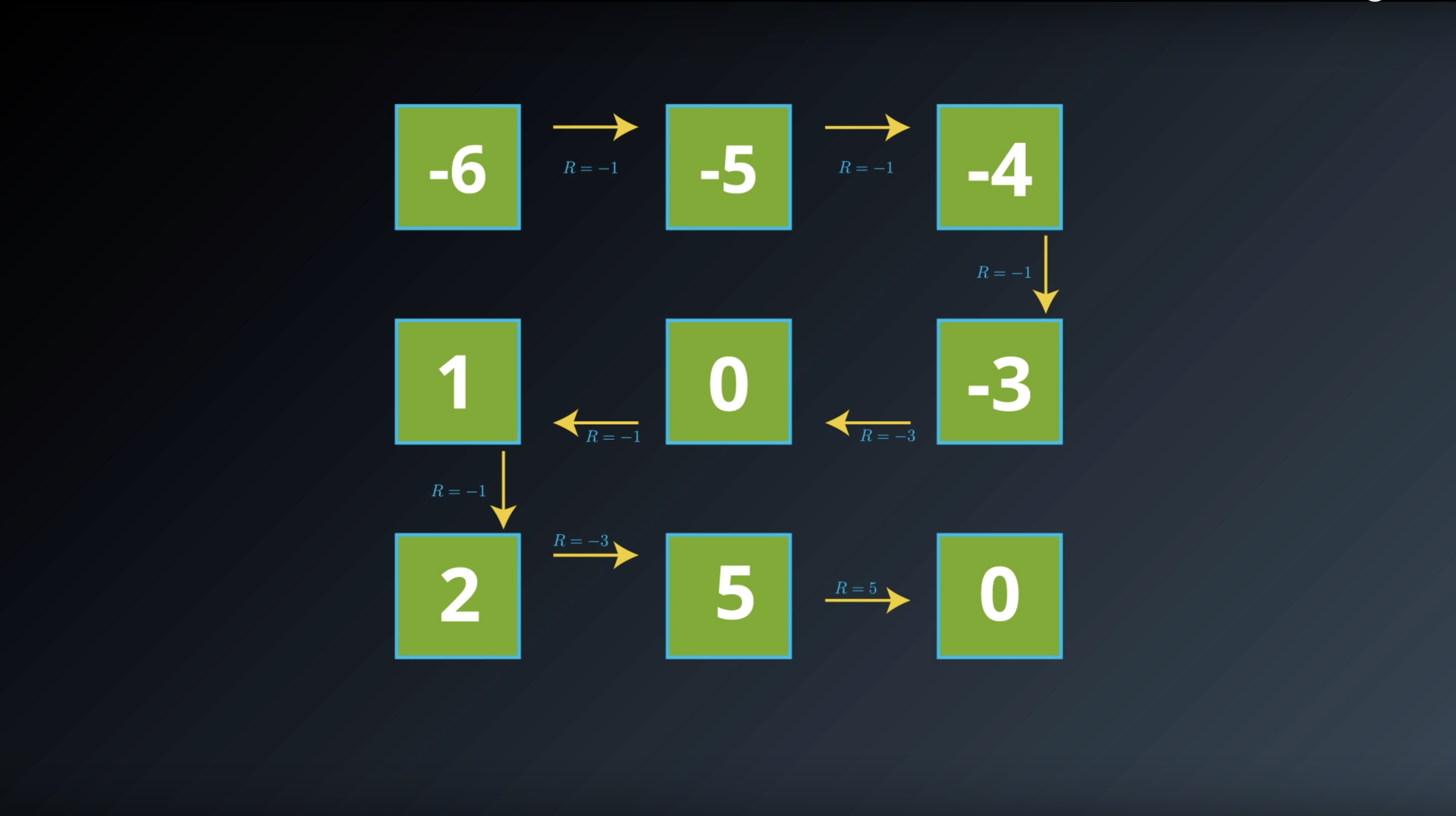
Image(filename='./images/1-2-3-5_state_function_value_of_all_states_are_calcurated_and saved_in_transition_table.png')

from IPython.display import Image
Image(filename='./images/1-2-3-6_state_function_value_of_terminal_state_is_0_and saved_in_transition_table.png')

from IPython.display import Image
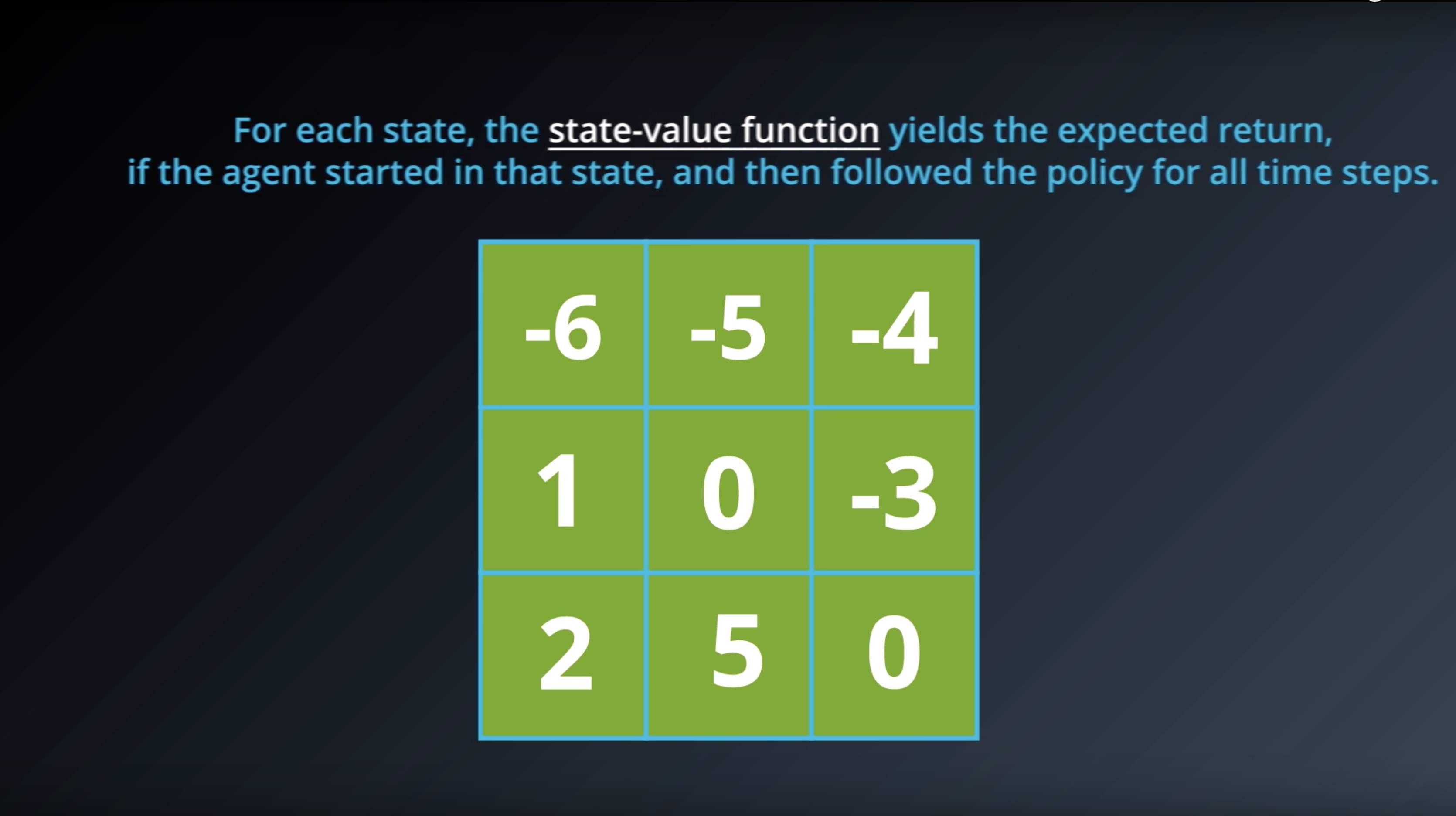
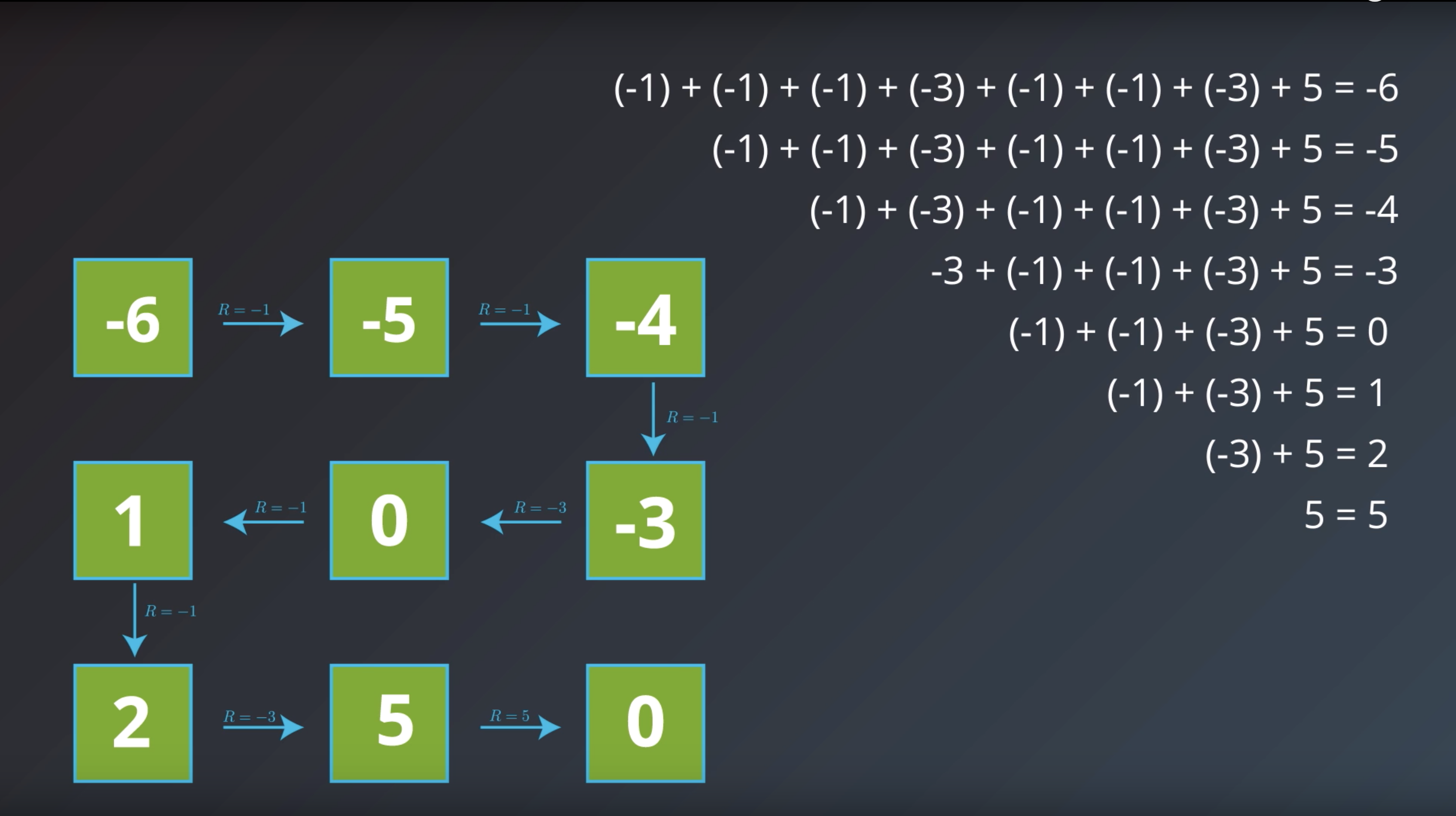
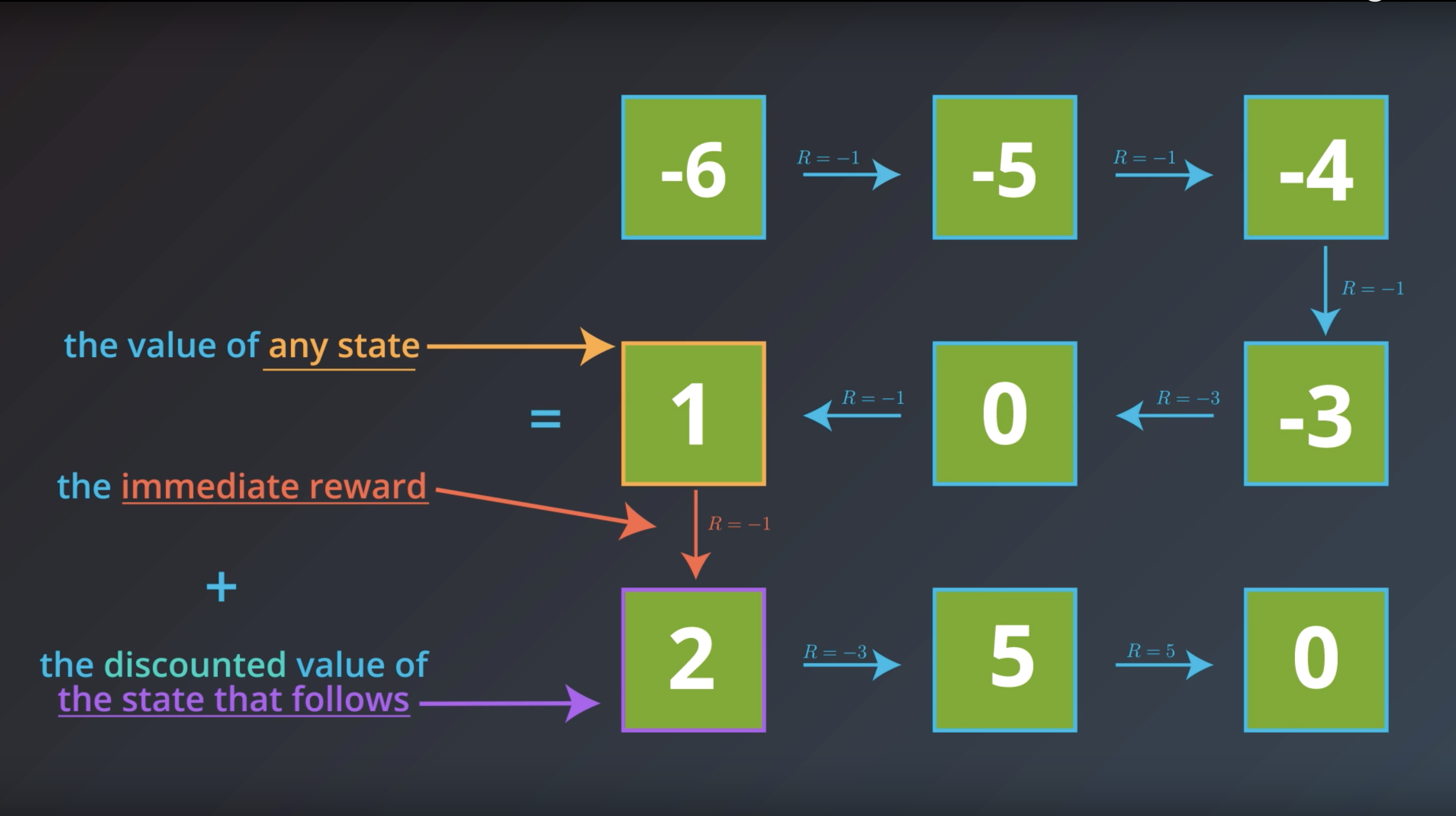
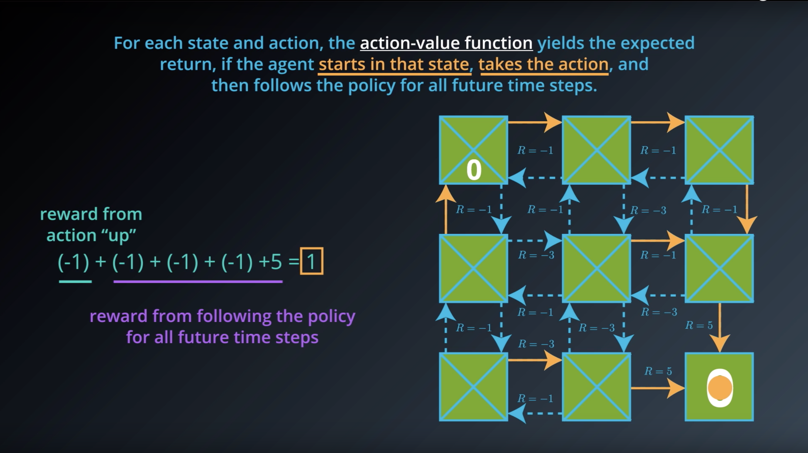
Image(filename='./images/1-2-3-7_state_function_yields_the_expected_return.png')

from IPython.display import Image
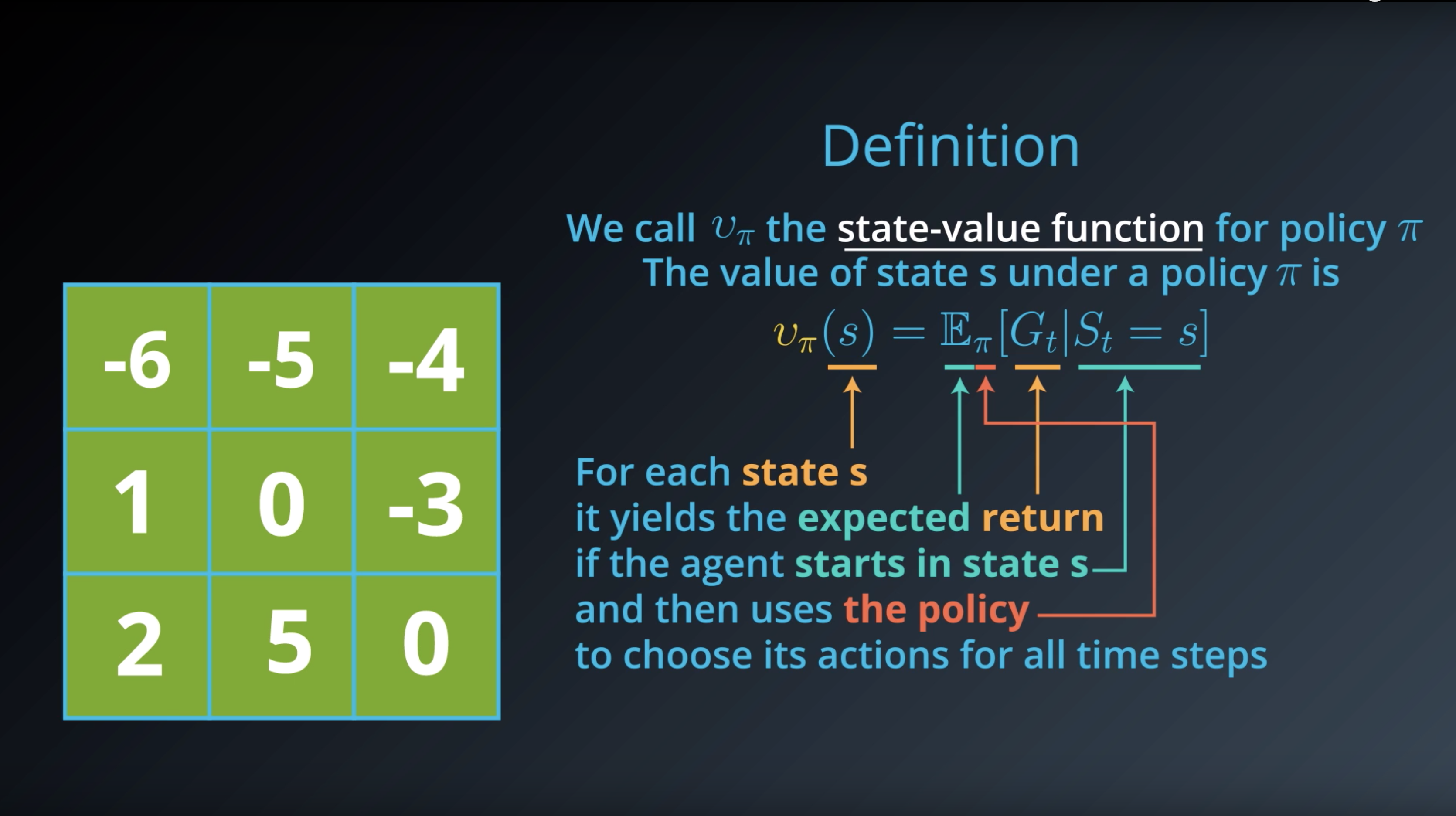
Image(filename='./images/1-2-3-8_definition_of_state_function.png')

Note #1: The notation Eπ[⋅] is borrowed from the suggested textbook. Eπ[⋅] is defined as the expected value of a random variable, given that the agent follows policy π.

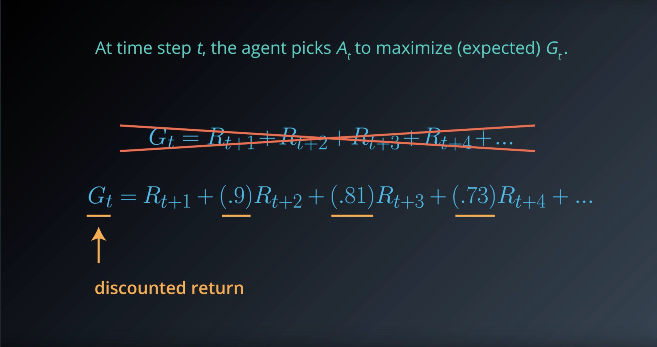
Note #2: In this blog, we will use “return” and “discounted return” interchangably. For an arbitrary time step t, both terms refer to Gt ≐ Rt+1 + γRt+2 + γ2Rt+3 + … = ∑ k=0 ∞ γk Rt+k+1 , where γ∈[0,1]. In particular, when we refer to “return”, it is not necessarily the case that γ=1, and when we refer to “discounted return”, it is not necessarily true that γ<1. (This also holds for the readings in the recommended Sutton’s textbook.)

1-2-4 : Bellman Equations

from IPython.display import Image
Image(filename='./images/1-2-4-1_bellman_equation_there_are_redundant_process_in_calcurating_each_expected_return.png')

from IPython.display import Image
Image(filename='./images/1-2-4-2_bellman_equation_calcurate_Gt_of_curret_state.png')

from IPython.display import Image
Image(filename='./images/1-2-4-3_bellman_equation_calcurate_Gt_of_curret_state_with_sum_of_future_rewards_and_immediate_return.png')

from IPython.display import Image
Image(filename='./images/1-2-4-4_bellman_equation_calcurate_Gt_of_curret_state_t-1.png')

from IPython.display import Image
Image(filename='./images/1-2-4-5_bellman_equation_calcurate_Gt_of_curret_state_t-1_with_sum_of_future_rewards_and_immediate_return.png')

from IPython.display import Image
Image(filename='./images/1-2-4-6_bellman_equation_calcurate_Gt_of_curret_state_and_save_it.png')

from IPython.display import Image
Image(filename='./images/1-2-4-7_bellman_equation_calcurate_Gt_of_all_states.png')

from IPython.display import Image
Image(filename='./images/1-2-4-8_bellman_equation_how_to_calcurate.png')

from IPython.display import Image
Image(filename='./images/1-2-3-8_definition_of_state_function.png')

from IPython.display import Image
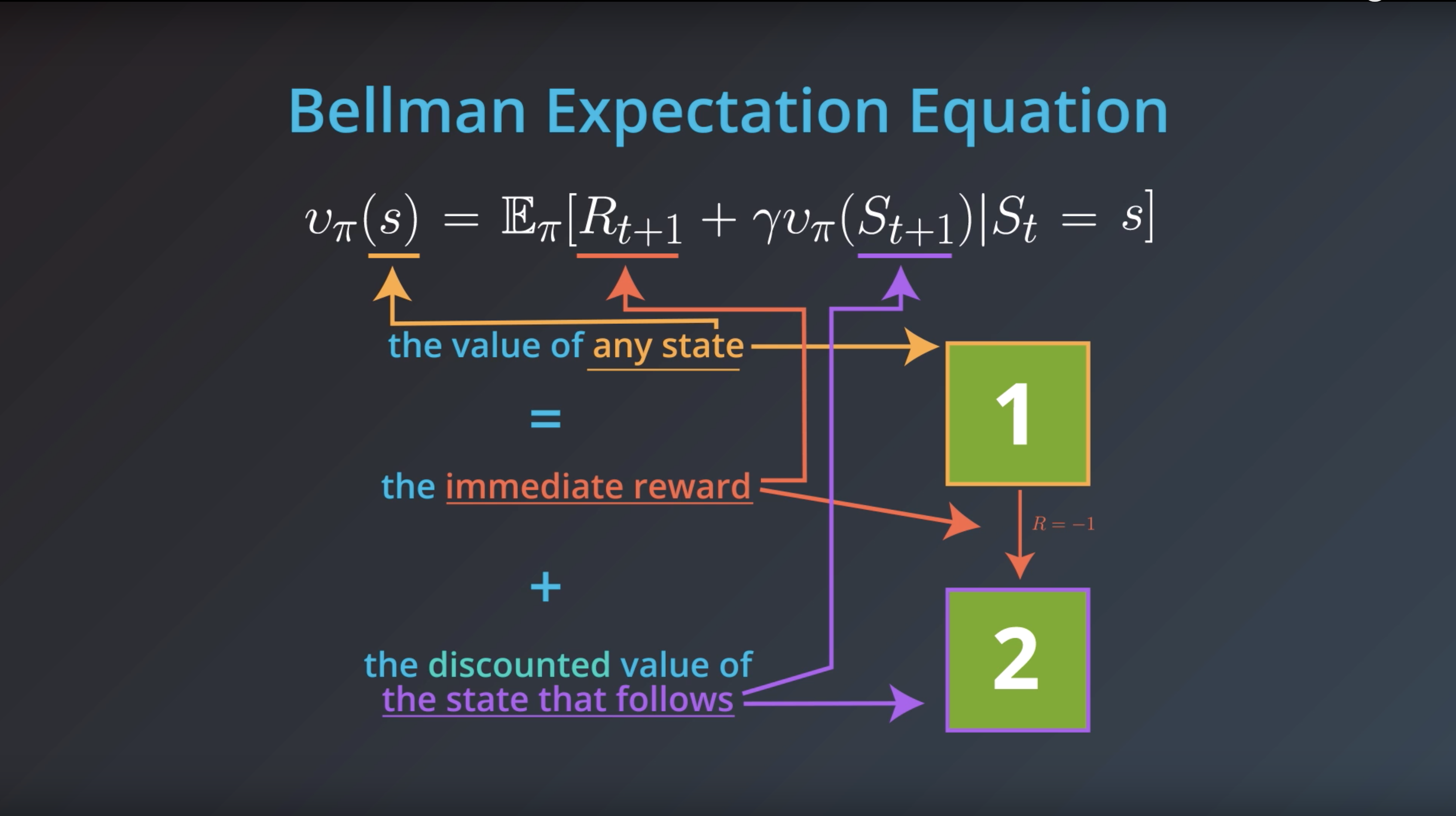
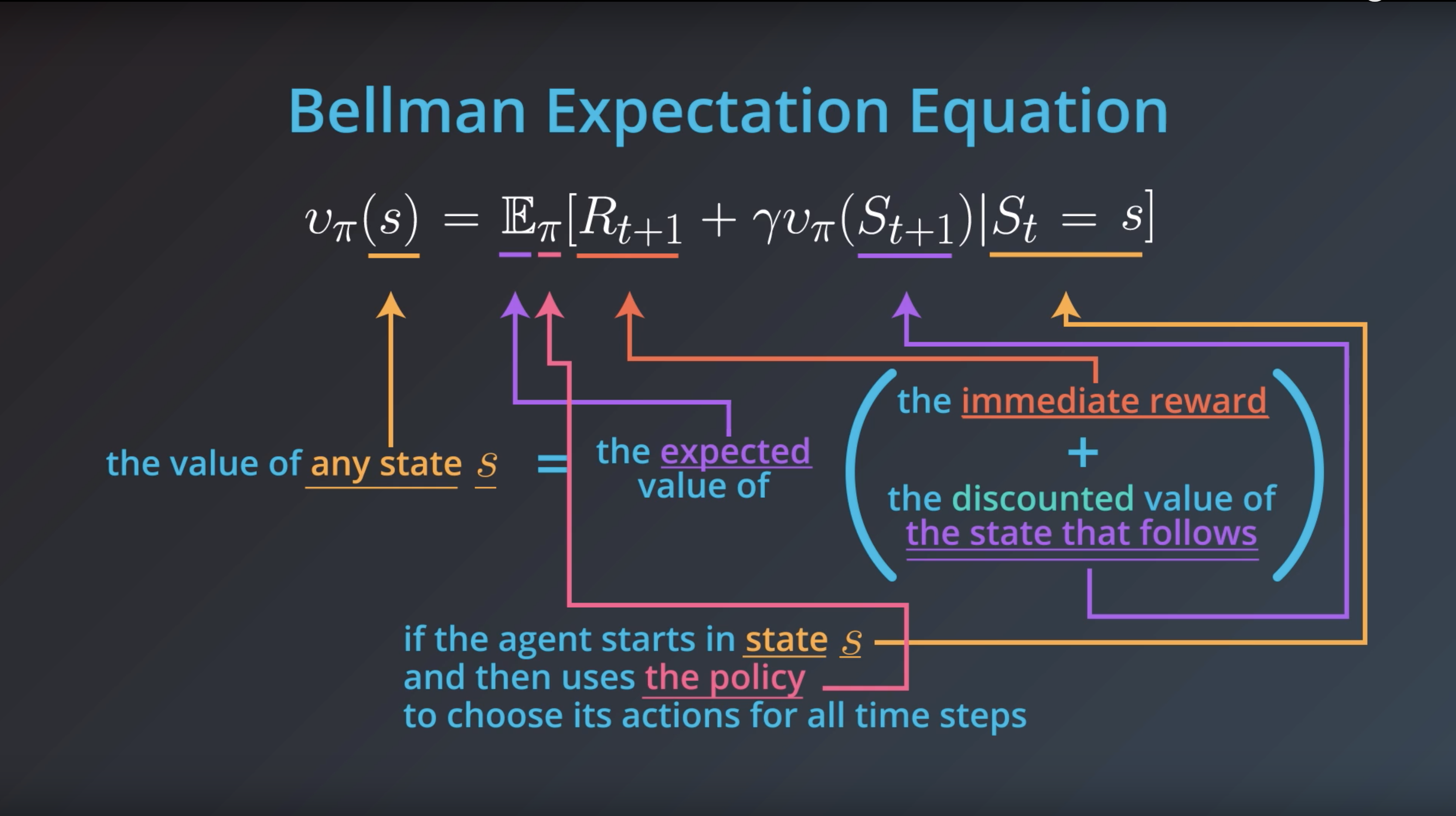
Image(filename='./images/1-2-4-9_bellman_expectatoin_equation_explanation.png')

from IPython.display import Image
Image(filename='./images/1-2-4-10_bellman_expectatoin_equation_detailed_explanation.png')

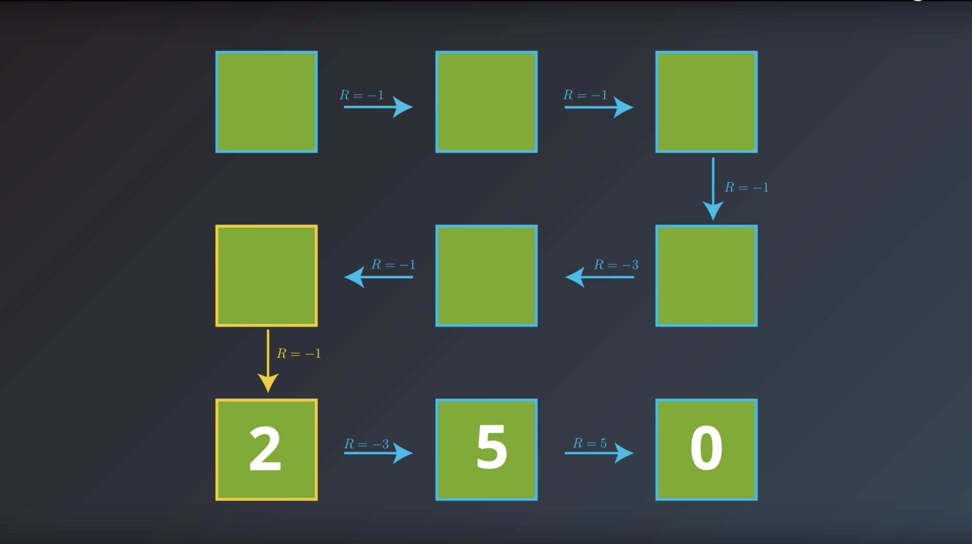
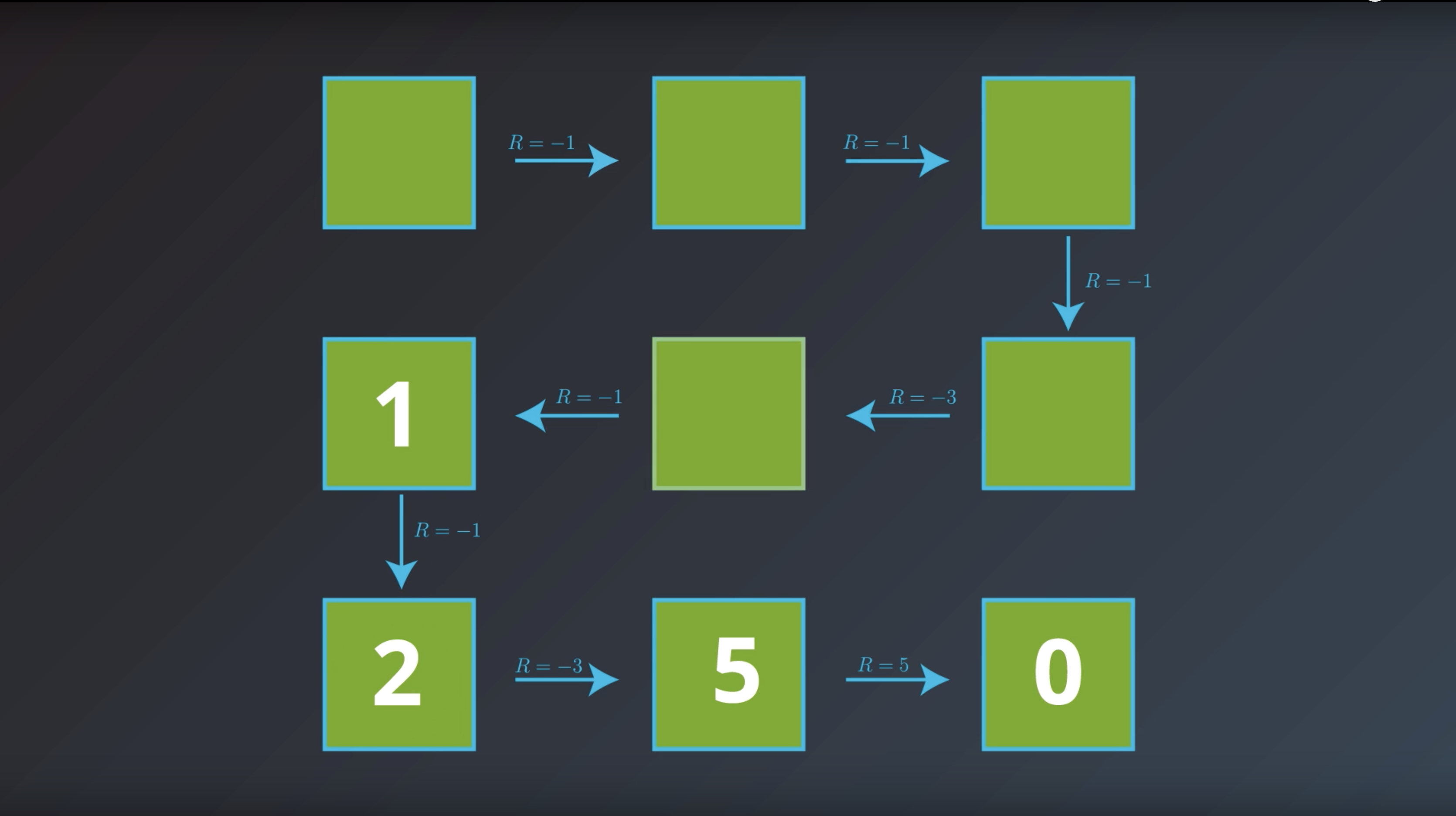
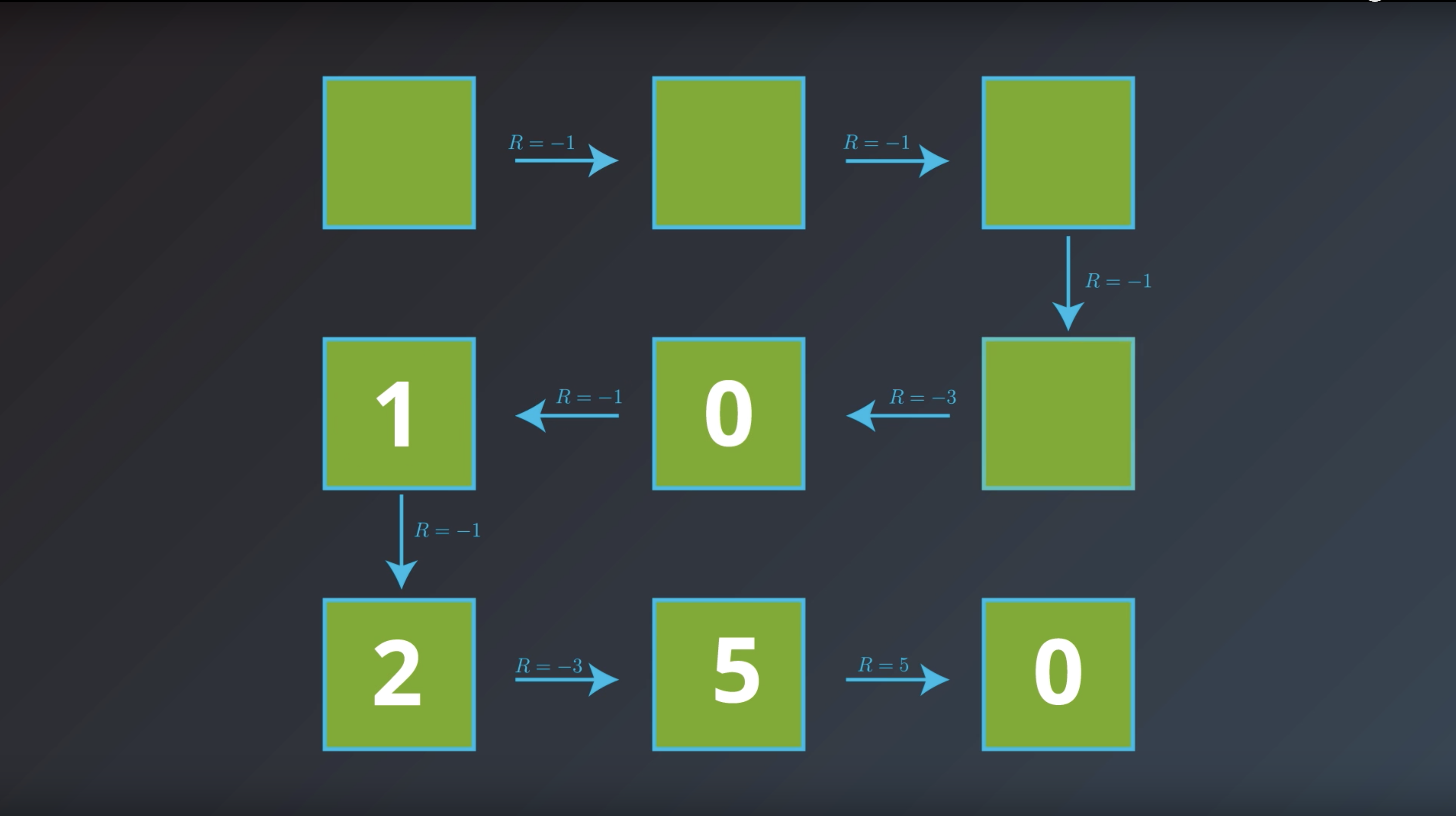
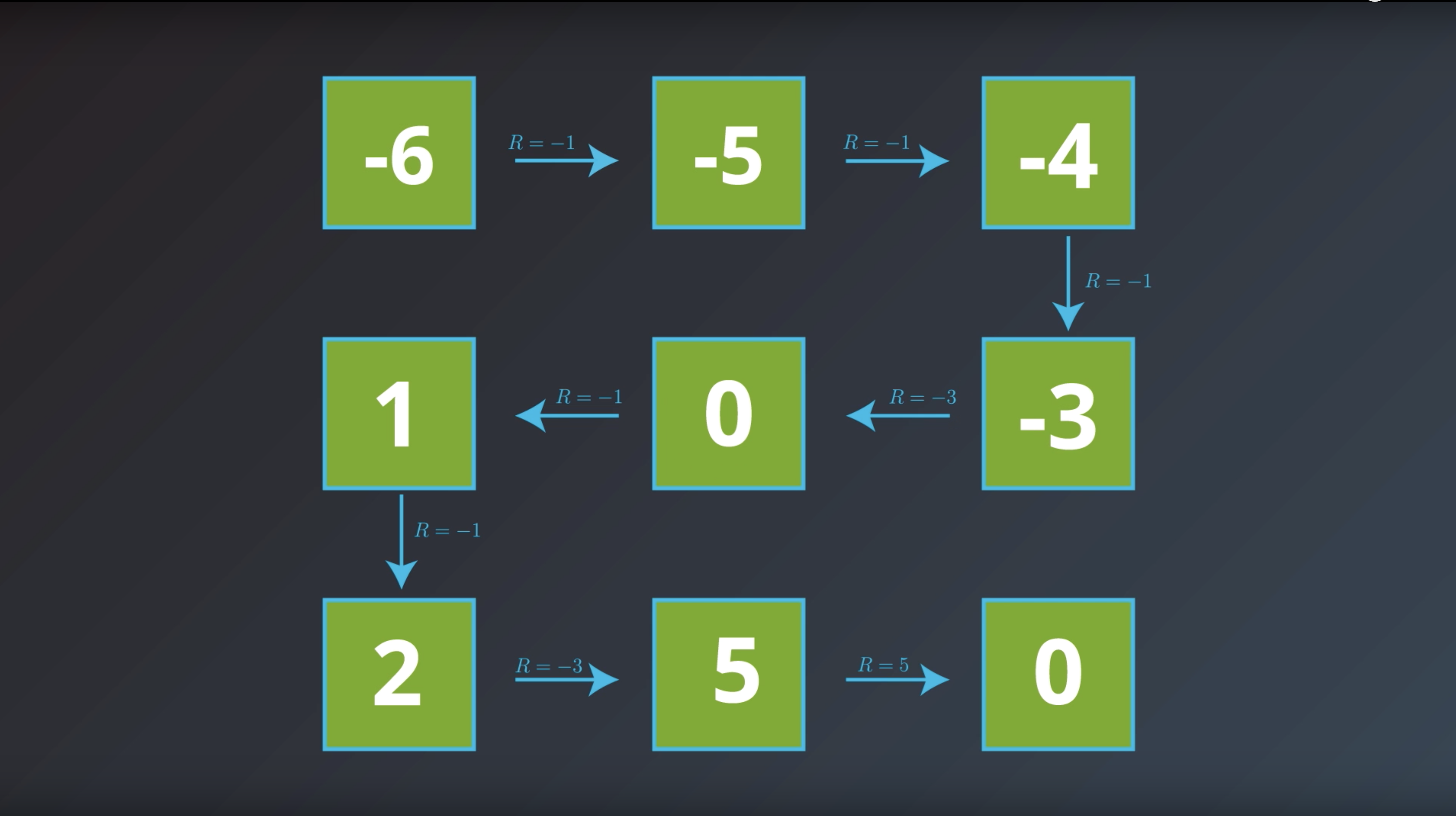
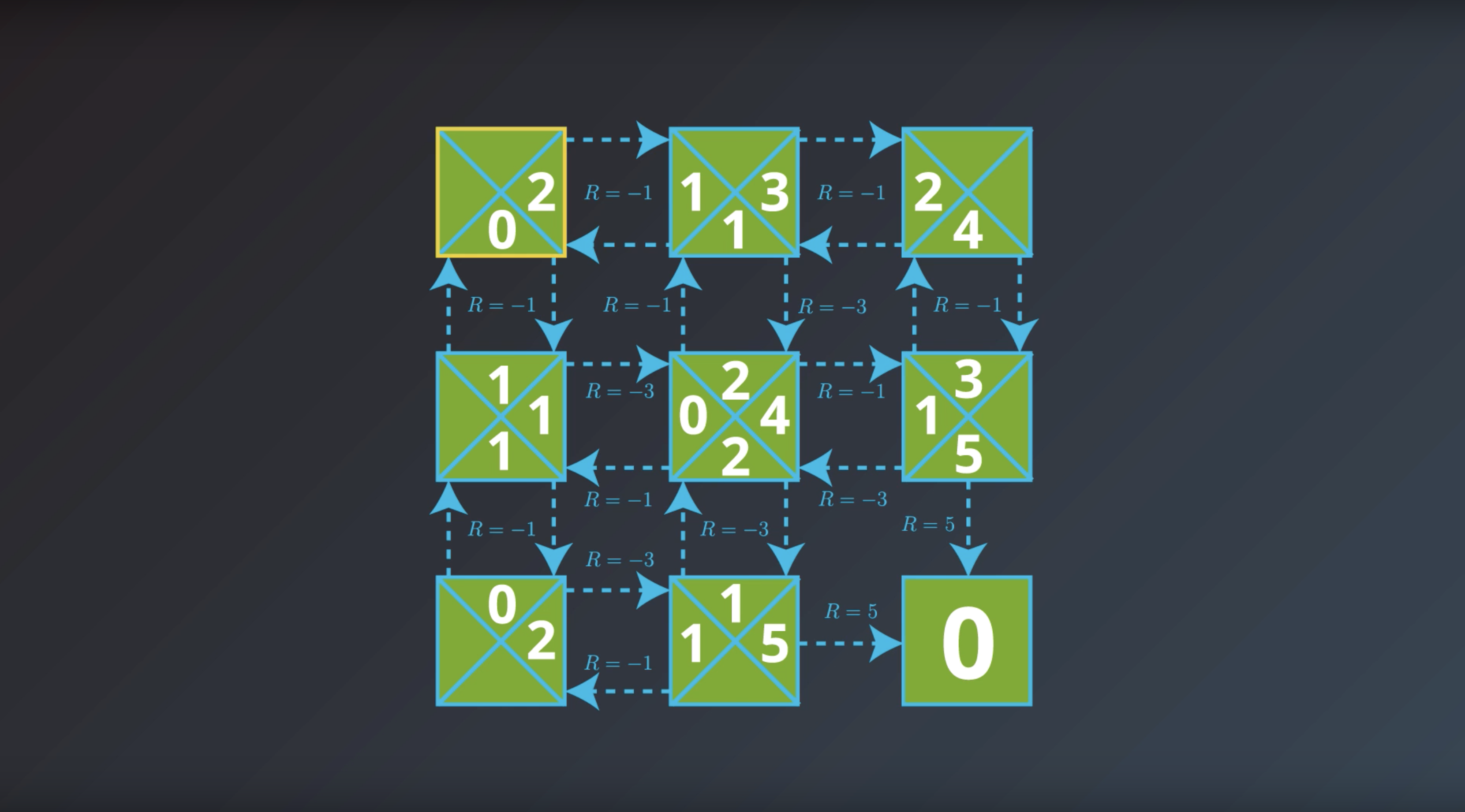
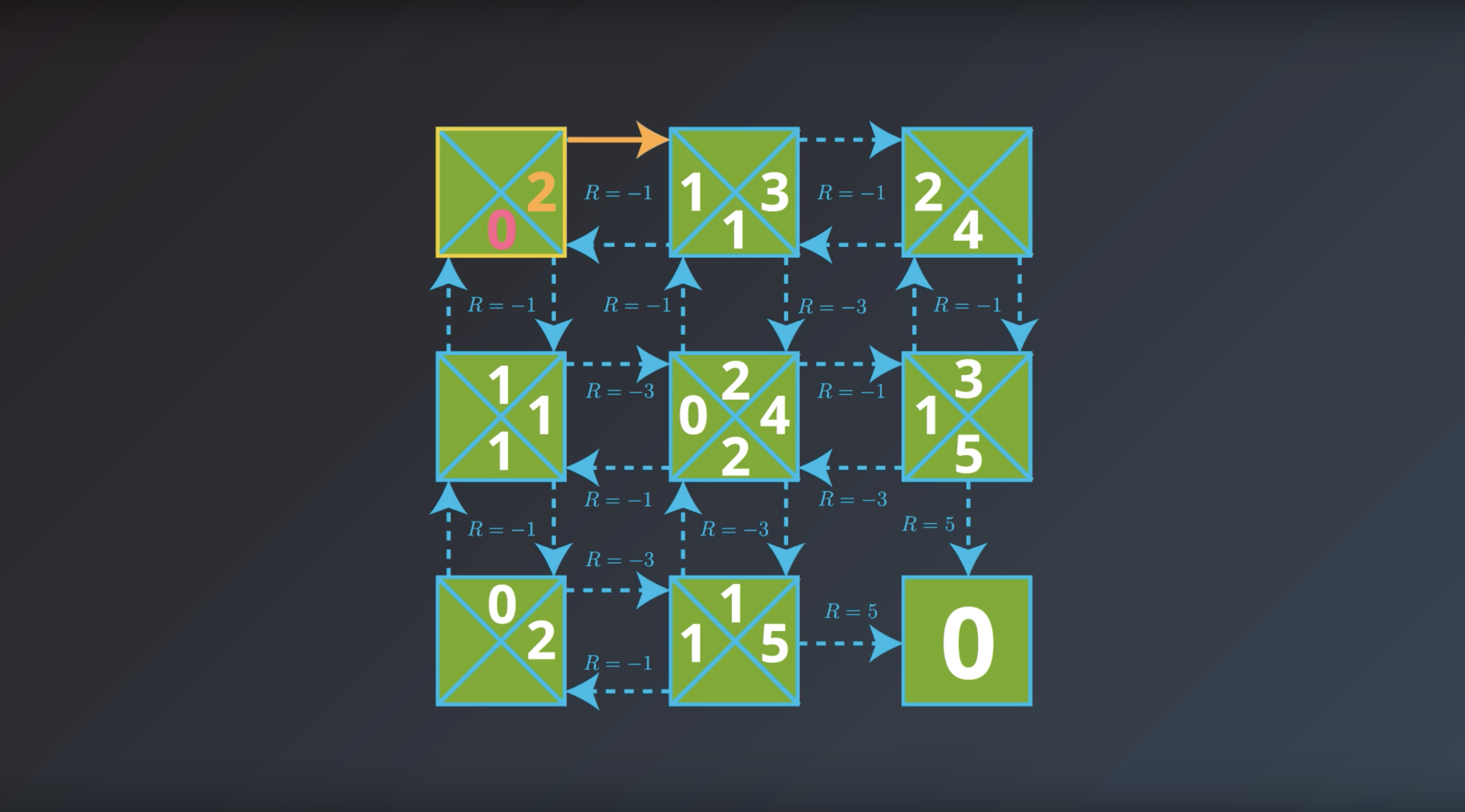
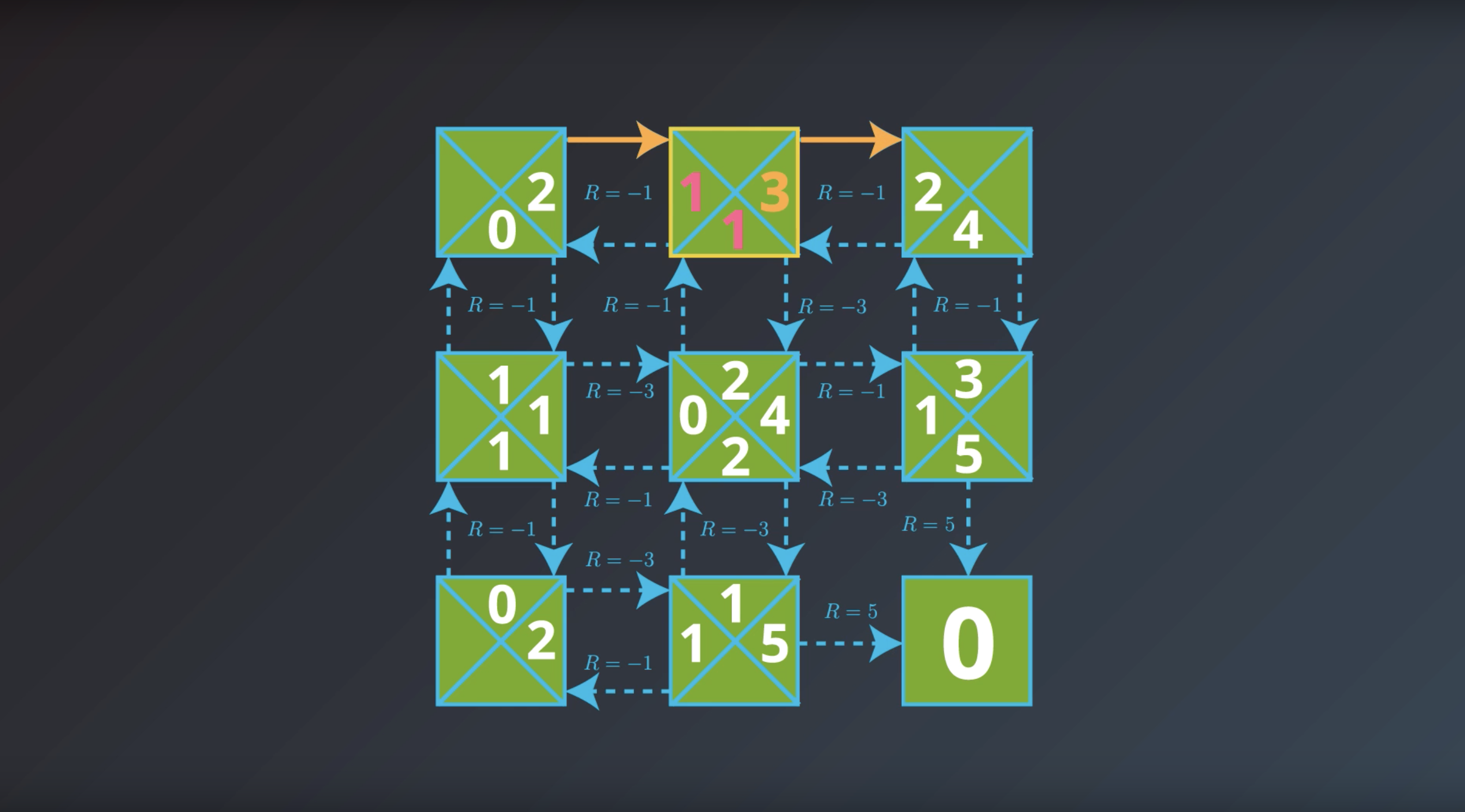
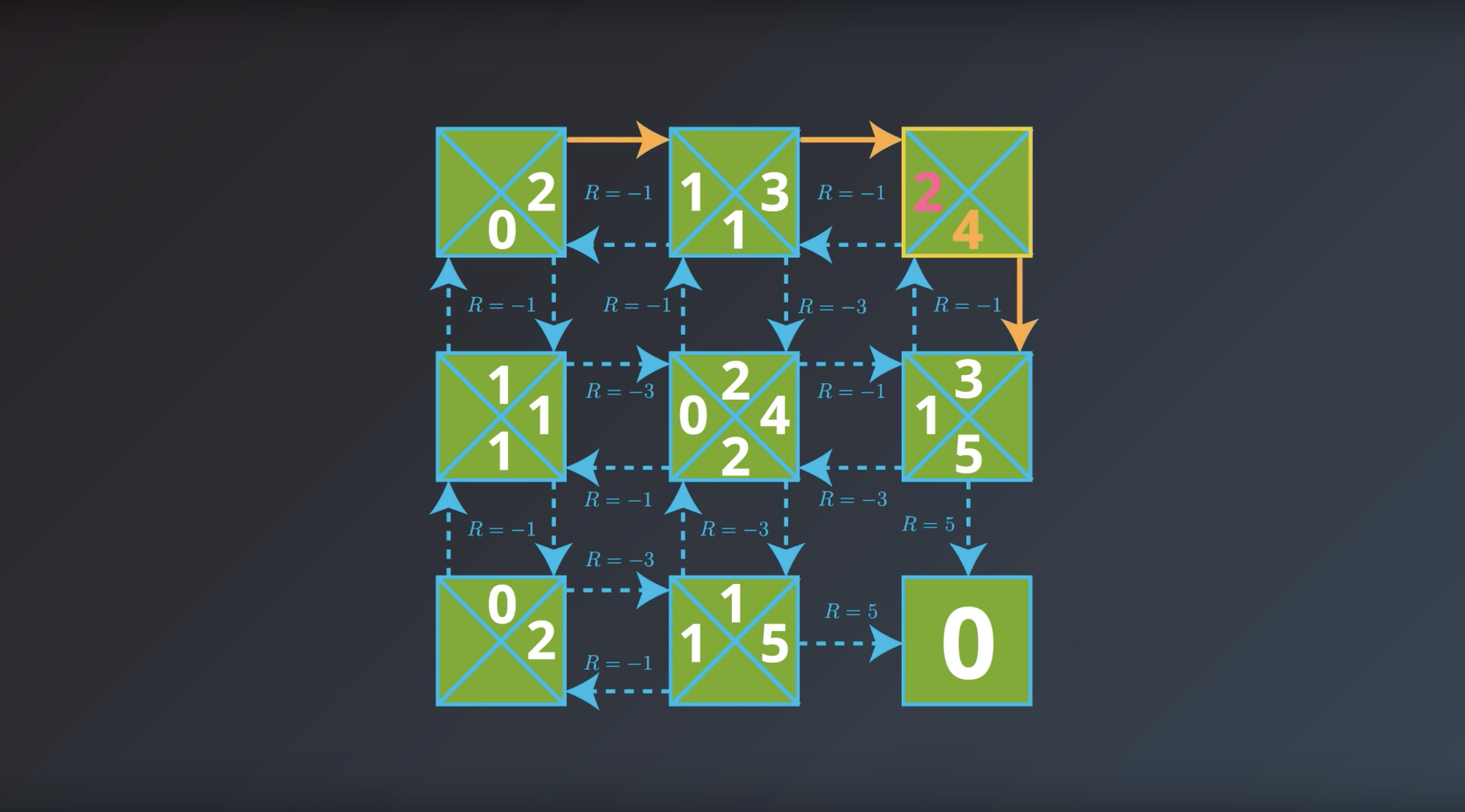
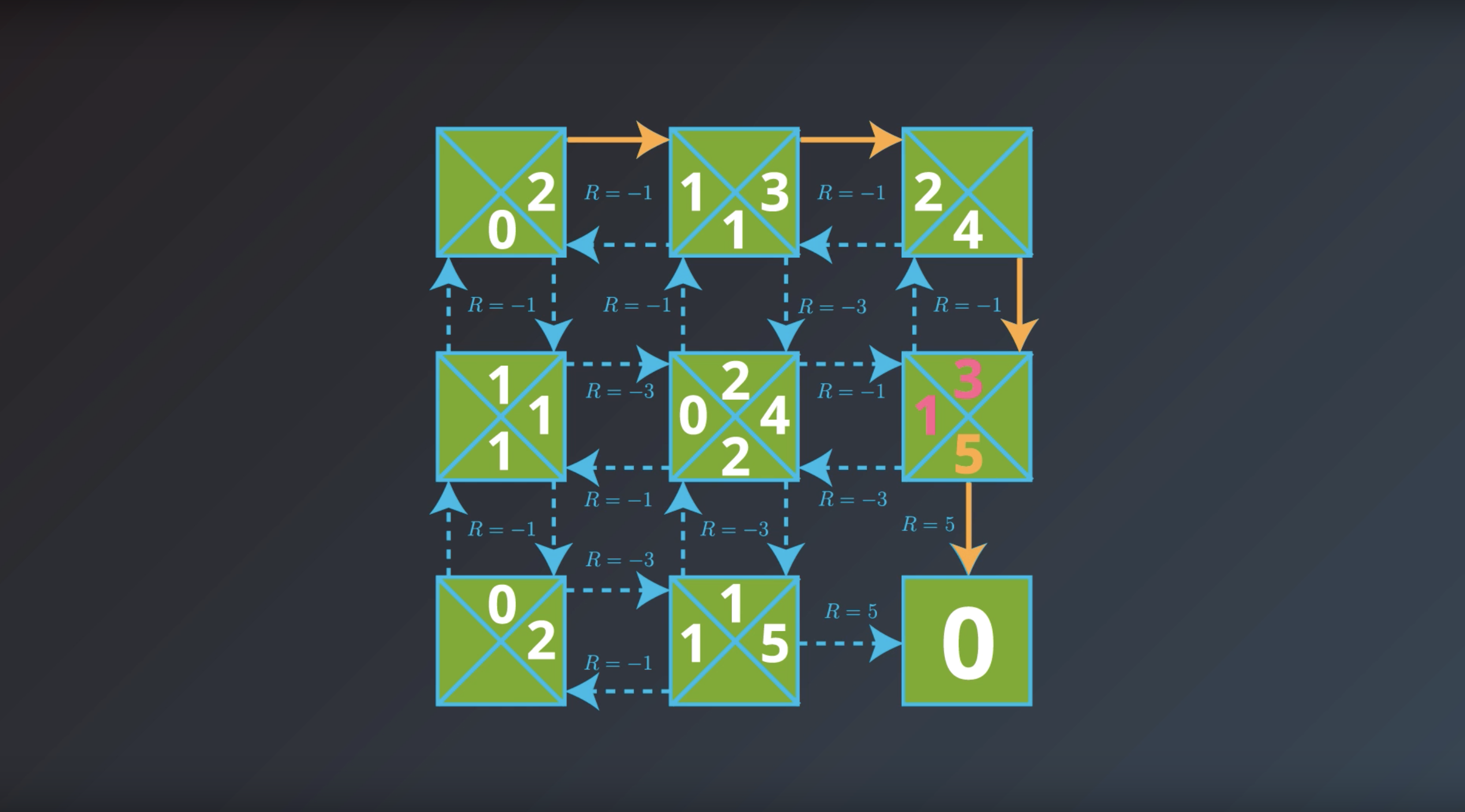
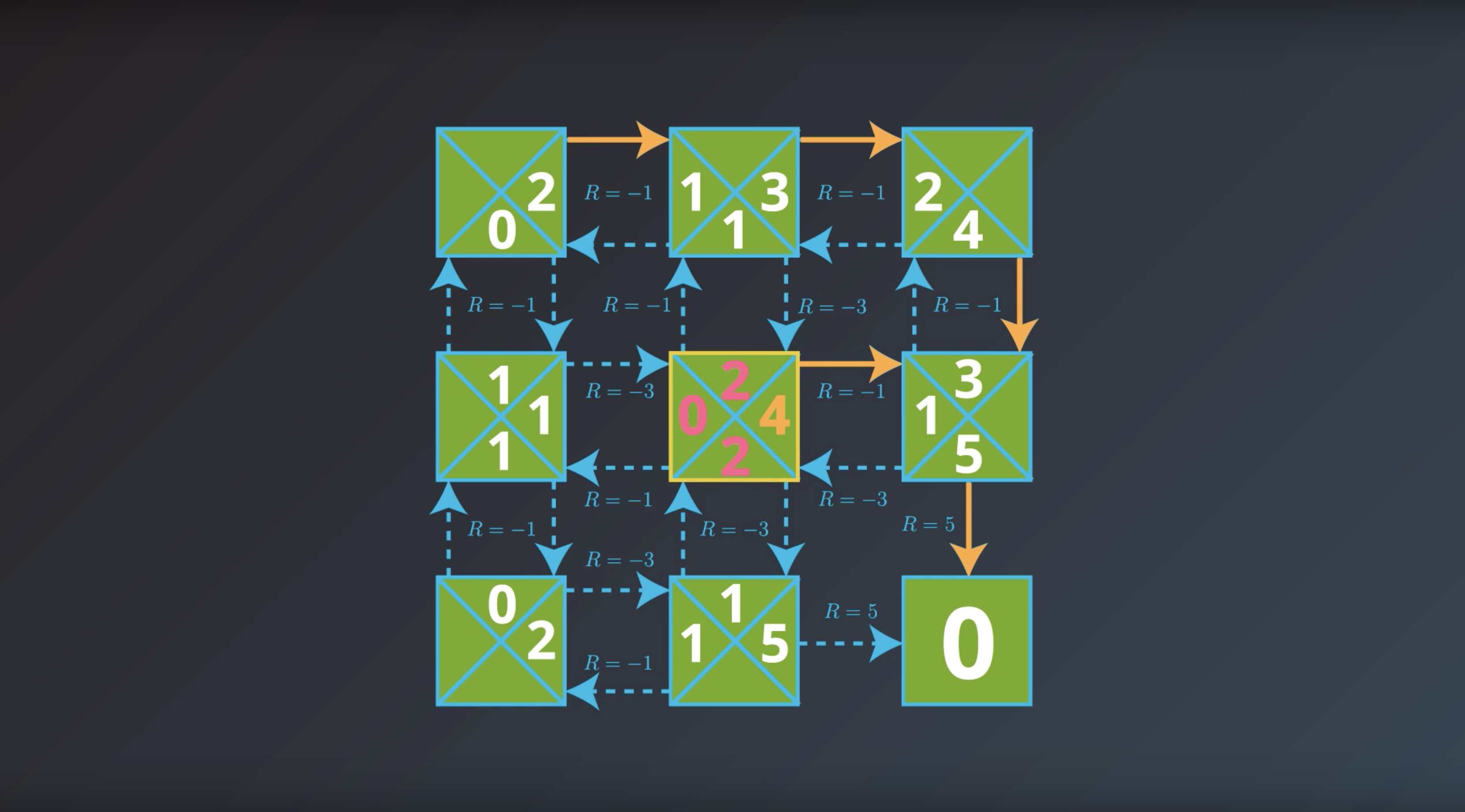
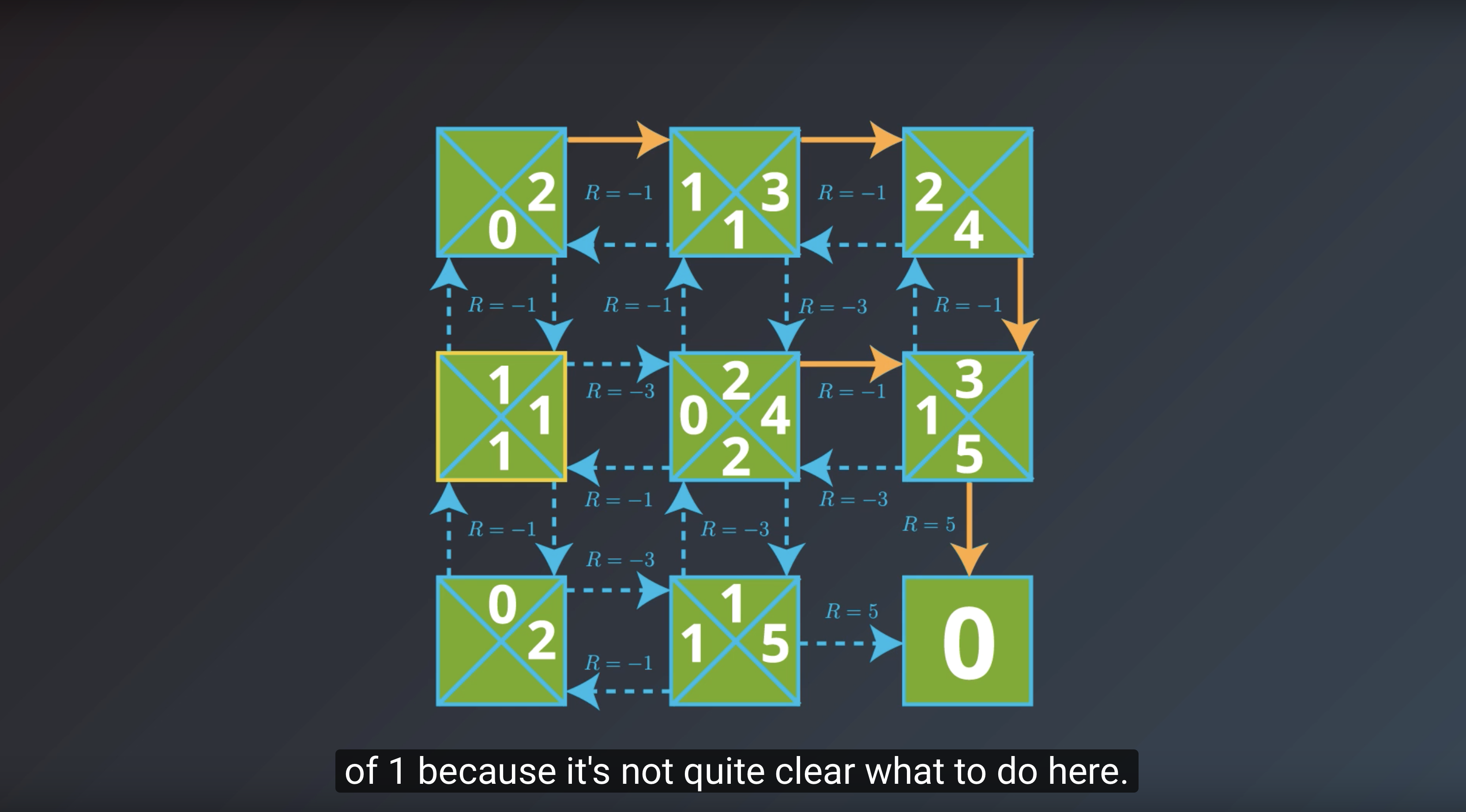
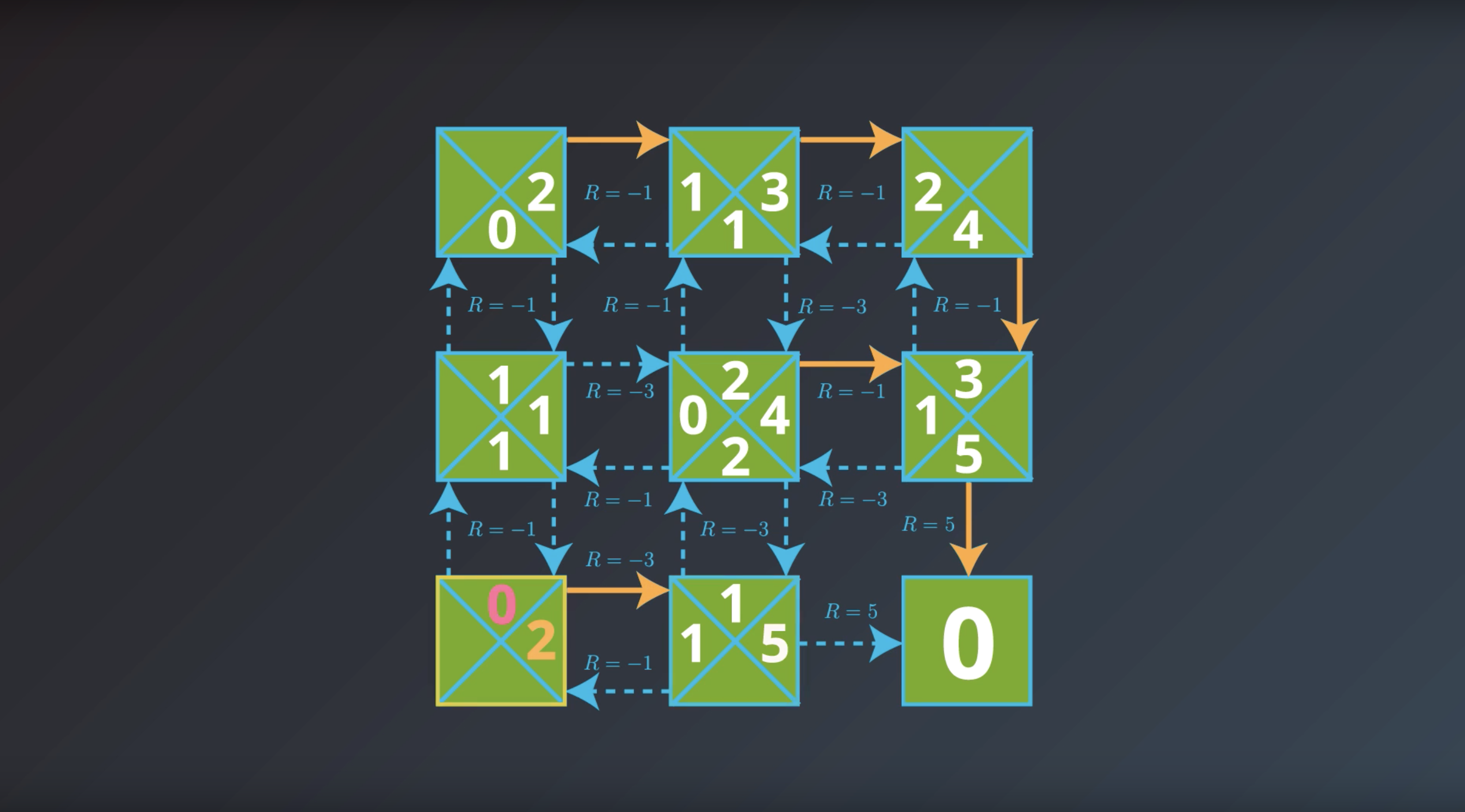
Quiz: State-Value Functions

In this quiz, you will calculate the value function corresponding to a particular policy.

Each of the nine states in the MDP is labeled as one of S+ ={s1,s2,…,s9}, where s9 is a terminal state.

Consider the (deterministic) policy that is indicated (in orange) in the figure below.

from IPython.display import Image
Image(filename='./images/1-2-4-11_quiz_state-value-function_gridworld_example.png')

The policy π is given by:

• π(s1)=right
• π(s2)=right
• π(s3)=down
• π(s4)=up
• π(s5)=right
• π(s6)=down
• π(s7)=right
• π(s8)=right

Recall that since s9 is a terminal state, the episode ends immediately if the agent begins in this state. So, the agent will not have to choose an action (so, we won’t include s9 in the domain of the policy), and vπ(s9)=0.

Take the time now to calculate the state-value function vπ that corresponds to the policy. (You may find that the Bellman expectation equation saves you a lot of work!)

Assume γ=1.

Once you have finished, use vπ to answer the questions below.

Question 1

What is vπ(s4)? Select the appropriate numerical value.

1. 2
2. -1
3. 0
4. 1
5. 2

Question 2

What is vπ(s1)? Select the appropriate numerical value.

1. 2
2. -1
3. 0
4. 1
5. 2

Question 3

Select the statements (listed above) that are true. (Select all that apply.)

• (1) vπ(s6) = -1 + vπ(s5)
• (2) vπ(s7) = -3 + vπ(s8)
• (3) vπ(s1) = -1 + vπ(s2)
• (4) vπ(s4) = -3 + vπ(s7)
• (5) vπ(s8) = -3 + vπ(s5)

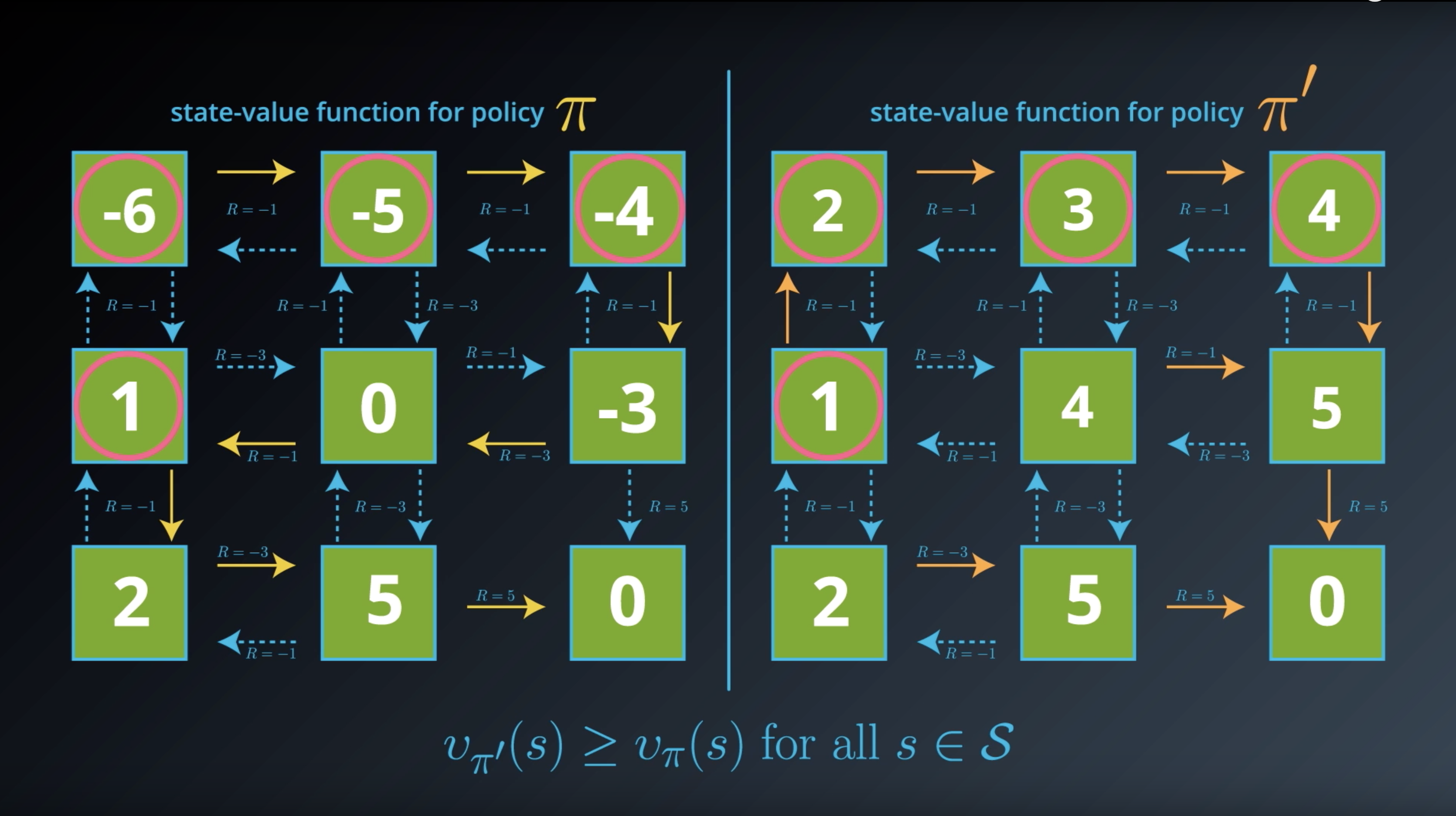
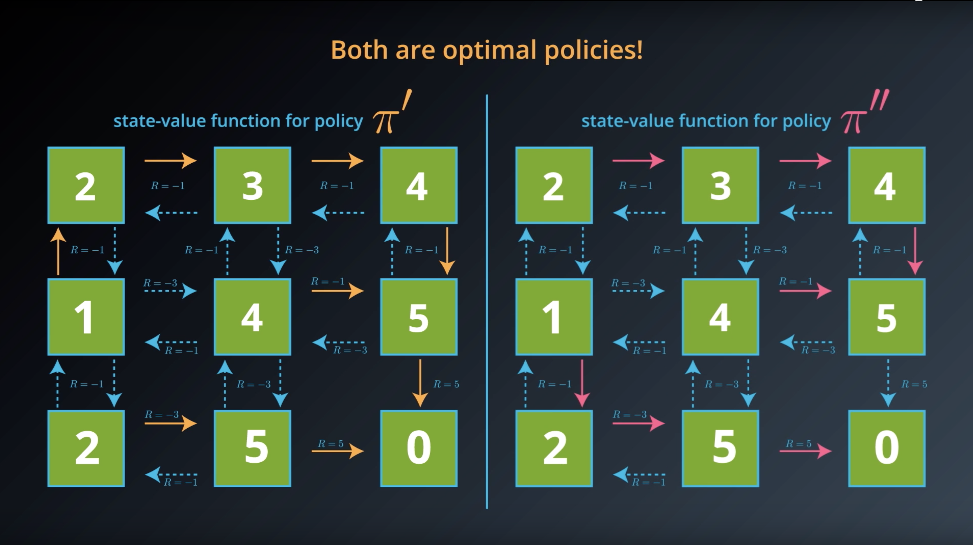
1-2-5 : Optimal Policy

from IPython.display import Image
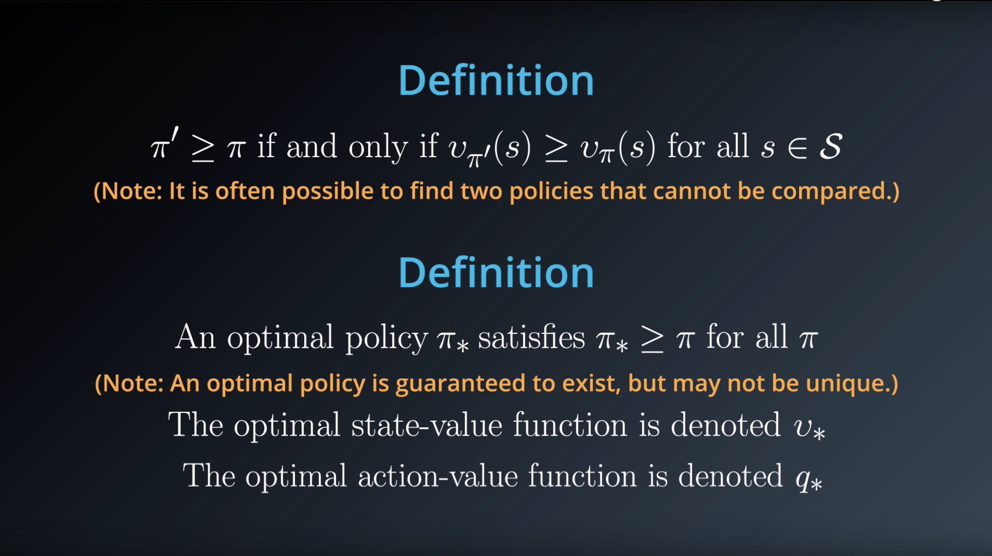
Image(filename='./images/1-2-5-1_optimal_policy_there_are_lots_of_policies.png')

from IPython.display import Image
Image(filename='./images/1-2-5-2_optimal_policy_all-of_values_of_policy_pi_prime_are_bigger_than_policy_pi.png')

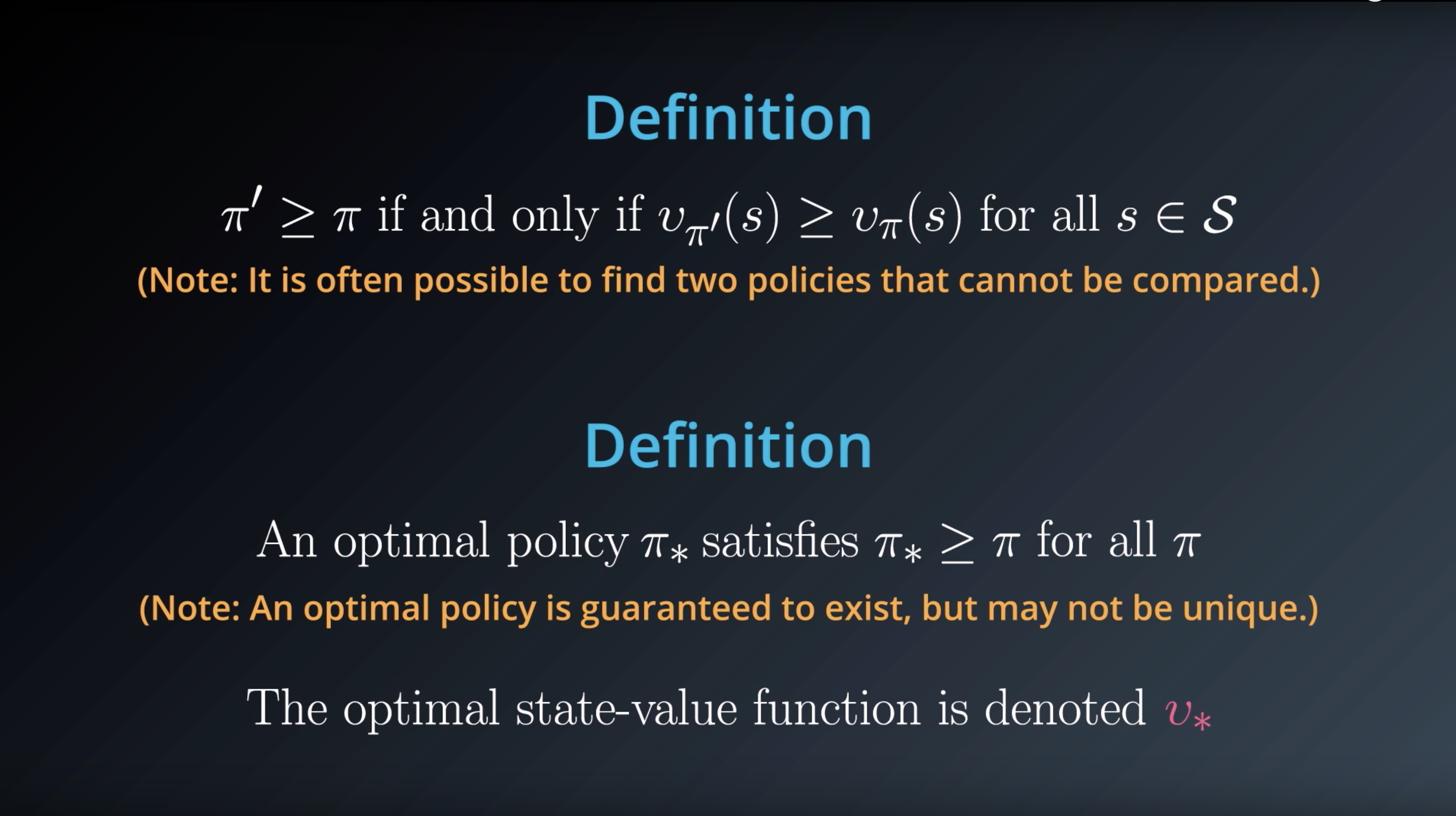
from IPython.display import Image
Image(filename='./images/1-2-5-3_optimal_policy_definition_and_notation_pi_star.png')

from IPython.display import Image
Image(filename='./images/1-2-5-4_optimal_policy_example.png')

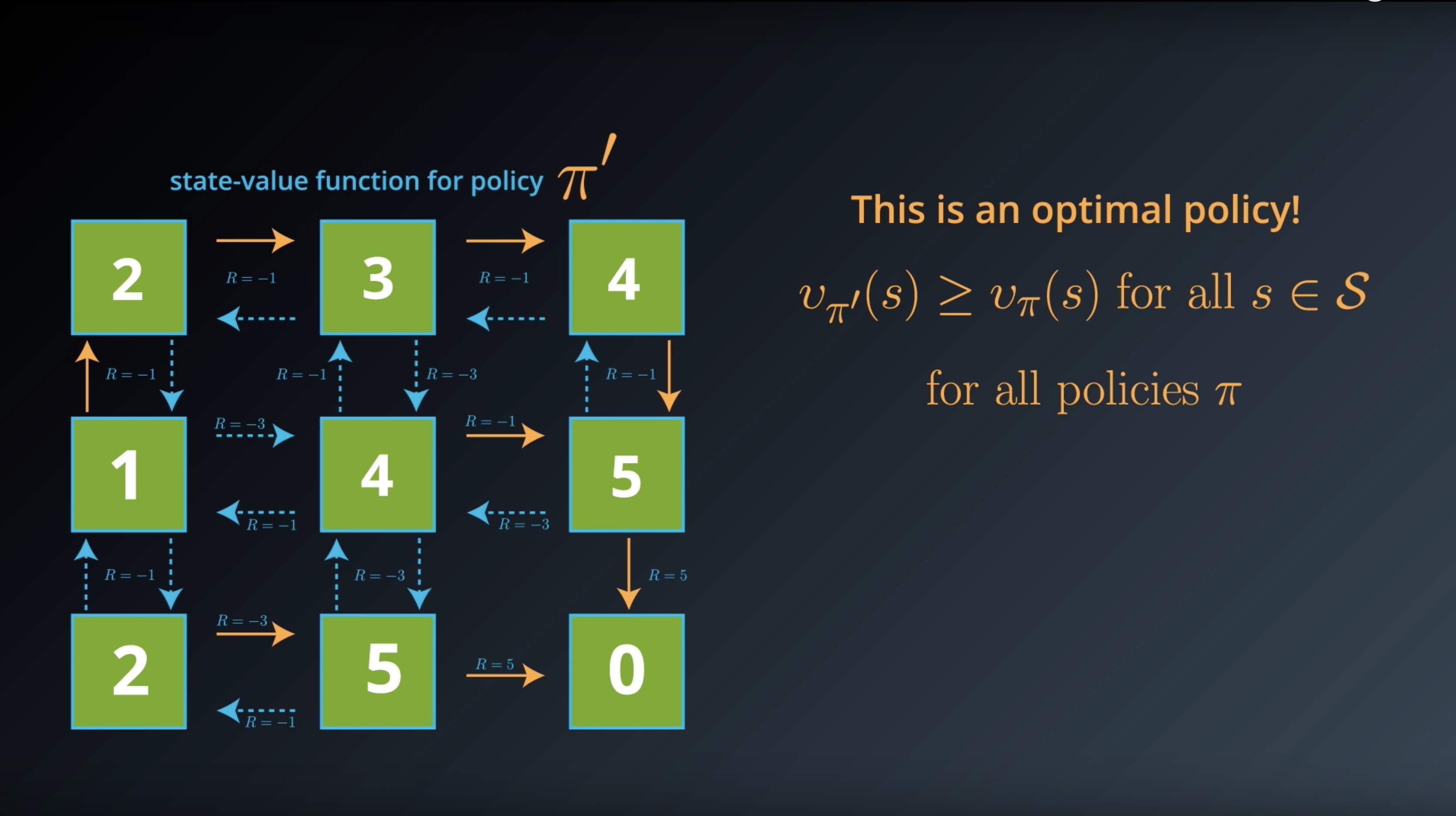
from IPython.display import Image
Image(filename='./images/1-2-5-5_optimal_policy_there_could_be_many_optimal_policies.png')

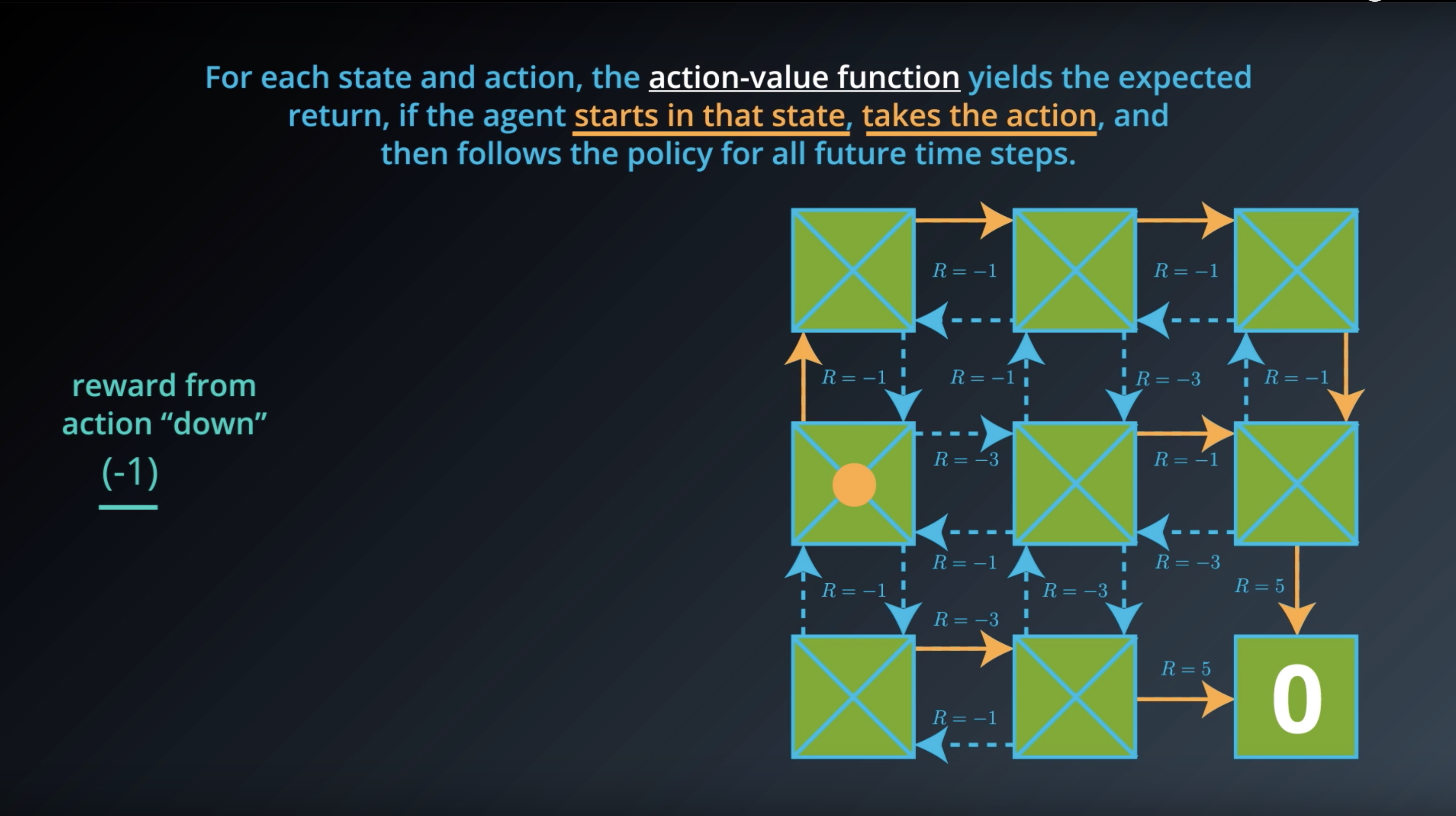
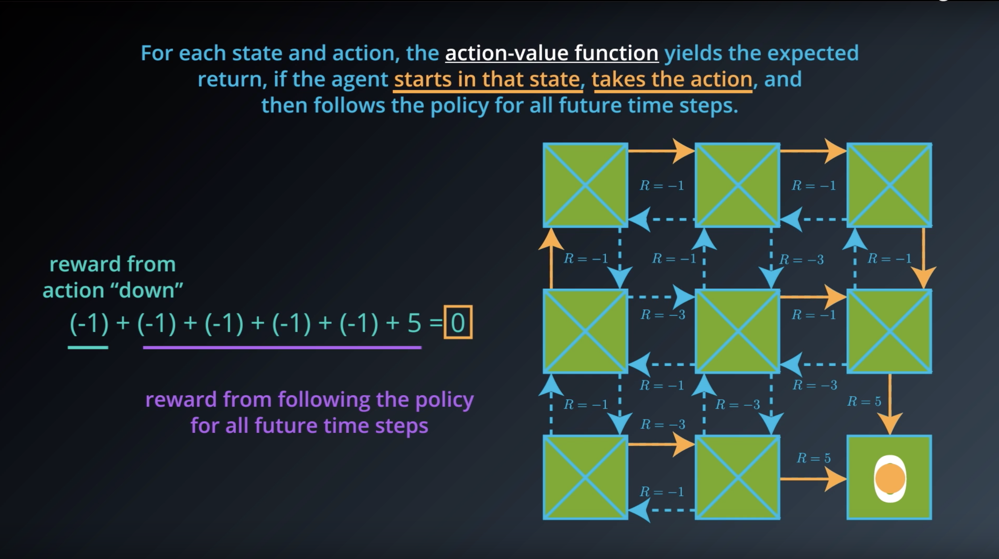
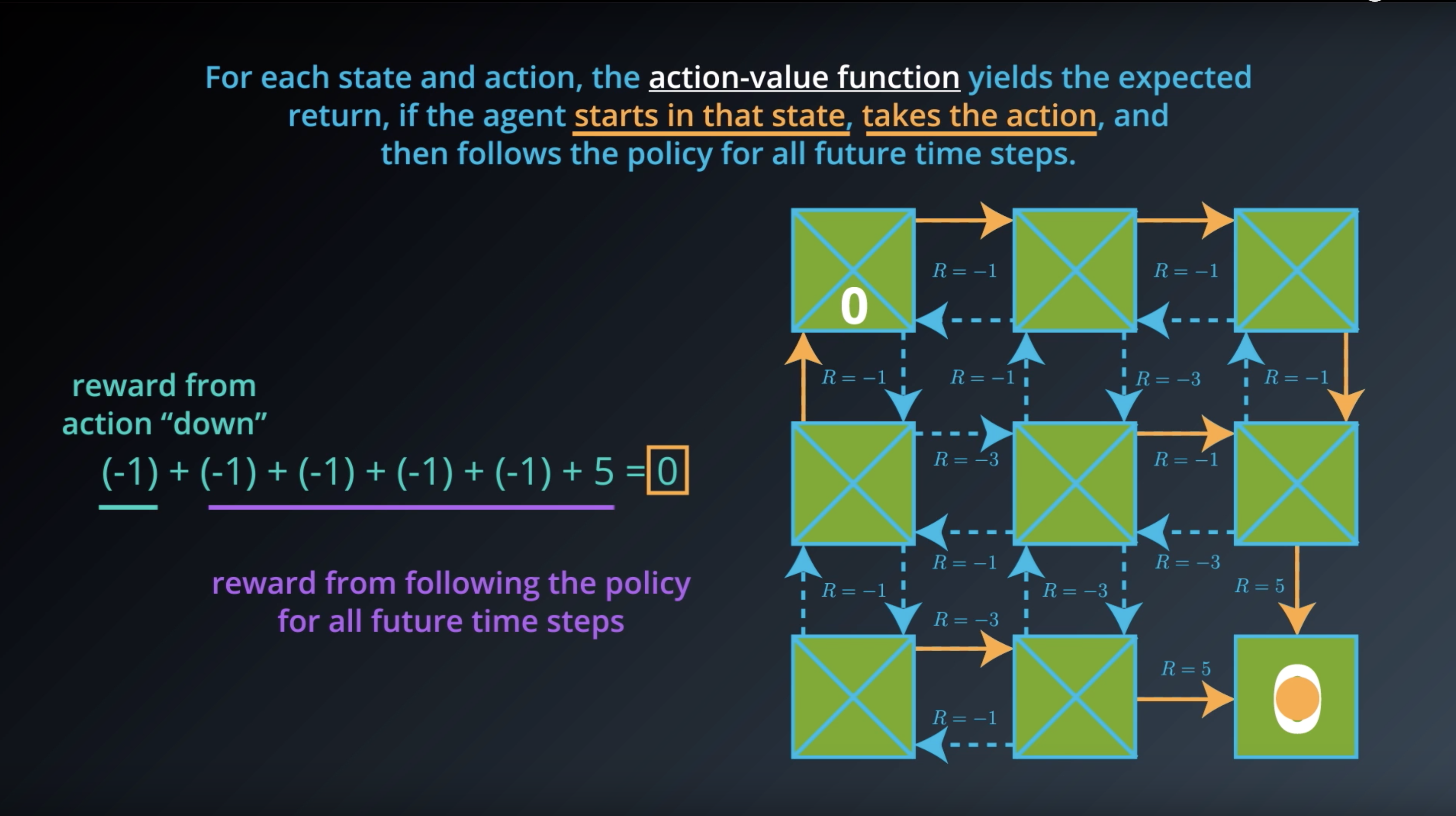
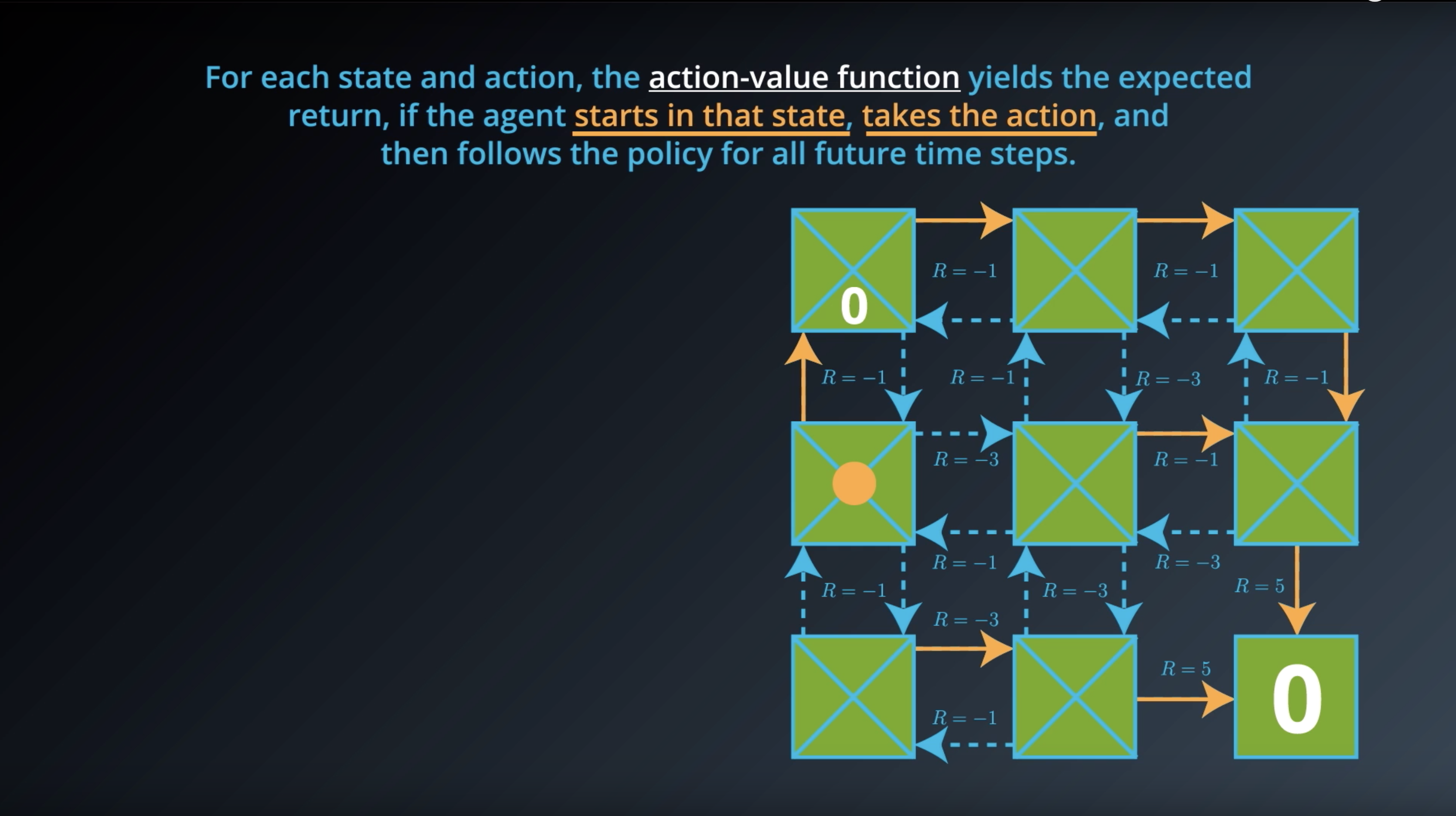
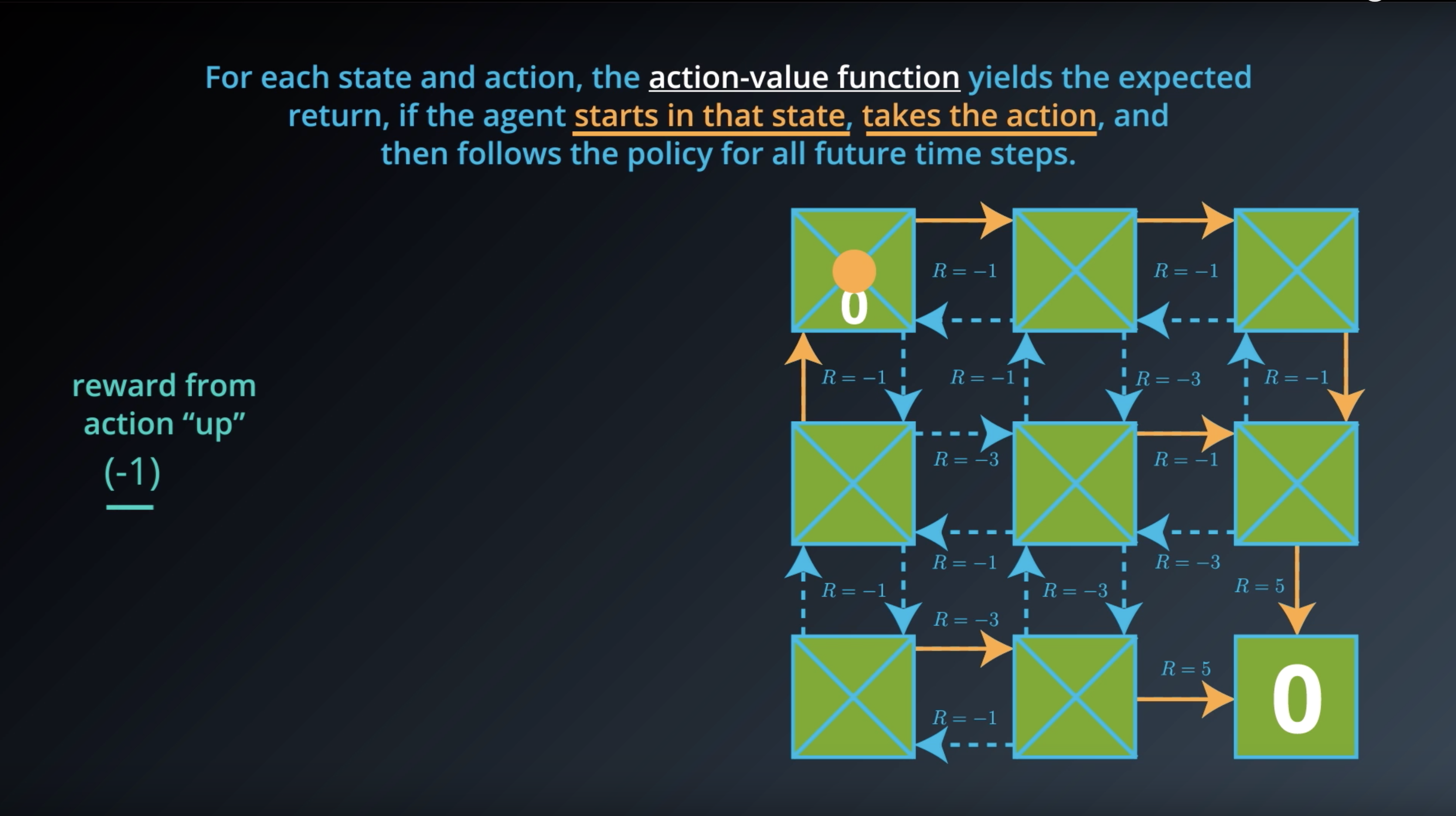
1-2-6 : Action-Value Functions

from IPython.display import Image
Image(filename='./images/1-2-6-1_action_value_function_definition.png')

from IPython.display import Image
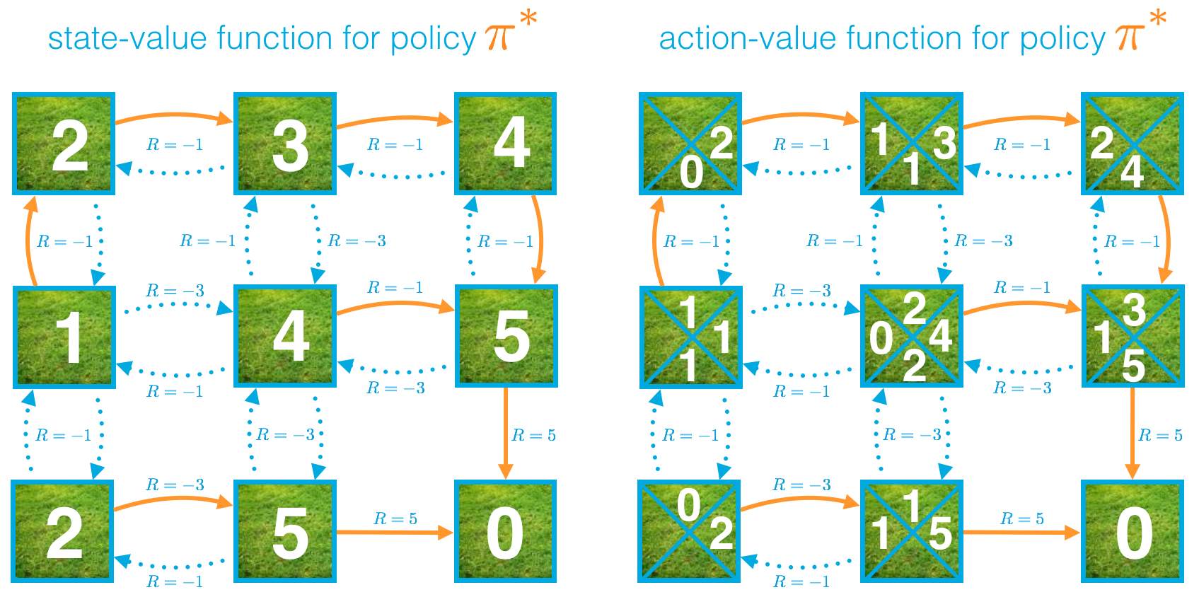
Image(filename='./images/1-2-6-2_state_value_function_vs_action_value_function.png')

from IPython.display import Image
Image(filename='./images/1-2-6-3_action_value_function_yield_expected_return_step1.png')

from IPython.display import Image
Image(filename='./images/1-2-6-4_action_value_function_yield_expected_return_step2.png')

from IPython.display import Image
Image(filename='./images/1-2-6-5_action_value_function_yield_expected_return_step3.png')

from IPython.display import Image
Image(filename='./images/1-2-6-6_action_value_function_yield_expected_return_step4.png')

from IPython.display import Image
Image(filename='./images/1-2-6-7_action_value_function_yield_expected_return_step1.png')

from IPython.display import Image
Image(filename='./images/1-2-6-8_action_value_function_yield_expected_return_step2.png')

from IPython.display import Image
Image(filename='./images/1-2-6-9_action_value_function_yield_expected_return_step3.png')

from IPython.display import Image
Image(filename='./images/1-2-6-10_action_value_function_yield_expected_return_step4.png')

from IPython.display import Image
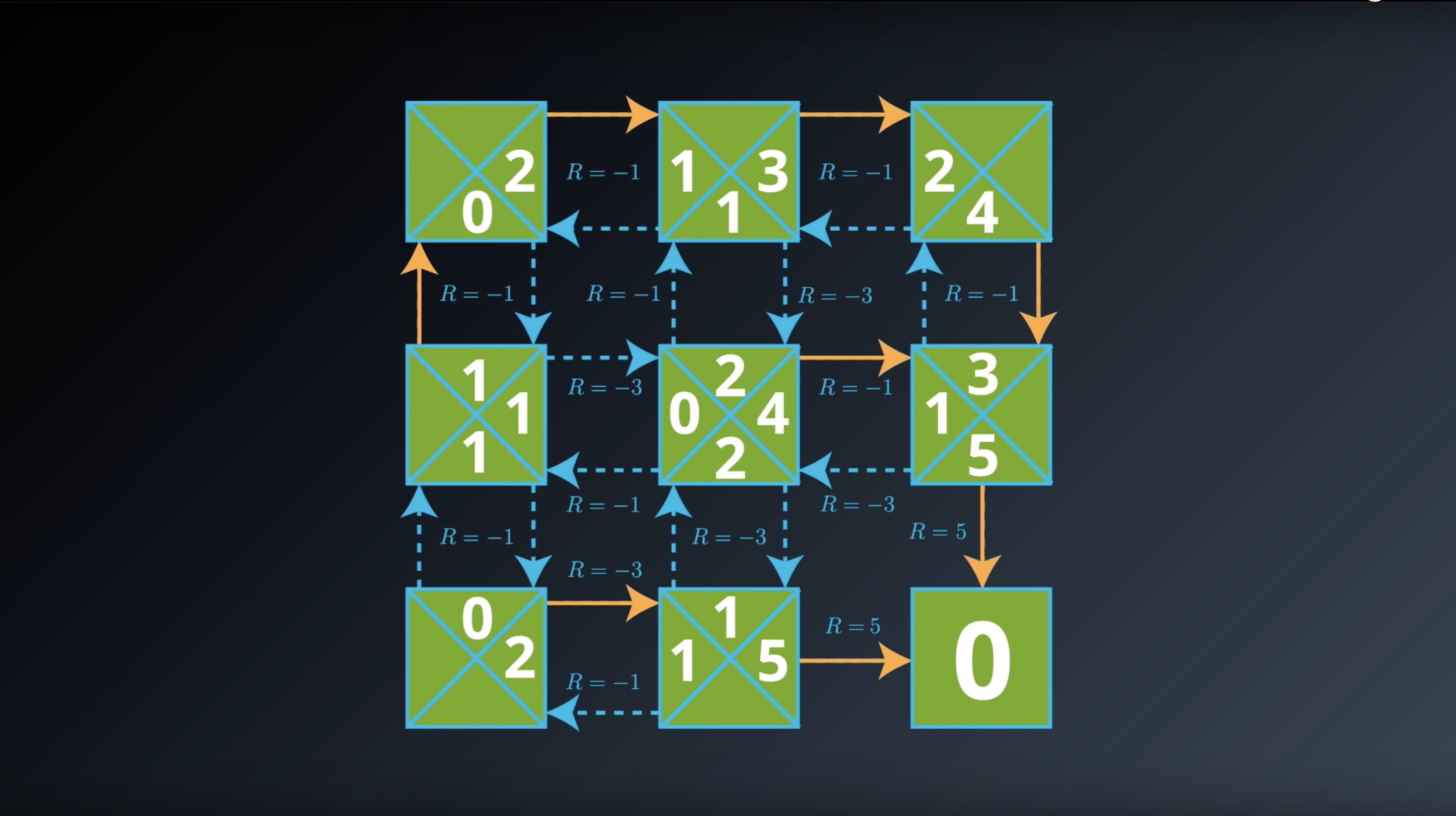
Image(filename='./images/1-2-6-11_action_value_function_yield_expected_return_all_done.png')

from IPython.display import Image
Image(filename='./images/1-2-6-12_optimal_action_value_function_q_star_definition.png')

Note: In this course, we will use “return” and “discounted return” interchangably. For an arbitrary time step t both refer to

Gt ≐ Rt+1 + γRt+2 + γ2Rt+3 + … = ∑ k=0 ∞ γkRt+k+1

where γ∈[0,1]. In particular, when we refer to “return”, it is not necessarily the case that γ=1, and when we refer to “discounted return”, it is not necessarily true that γ<1. (This also holds for the readings in the recommended Sutton’s textbook.)

Quiz: Action-Value Functions

from IPython.display import Image
Image(filename='./images/1-2-6-13_Quiz_Action-Value-Functions.png')

Question 1

True or False? : For a deterministic policy π,

vπ(s)=qπ(s,π(s))

holds for all s∈S.

Feel free to use the state-value and action-value functions (for an example deterministic policy) above to answer this question.

1-2-7 : Optimal Policies

from IPython.display import Image
Image(filename='./images/1-2-7-1_if_we_would_have_optimal_action_value_function_then_could_we_have_optimal_policy_?.png')

from IPython.display import Image
Image(filename='./images/1-2-7-2_yield_optimal_policy_step1.png')

from IPython.display import Image
Image(filename='./images/1-2-7-3_yield_optimal_policy_step2.png')

from IPython.display import Image
Image(filename='./images/1-2-7-4_yield_optimal_policy_step3.png')

from IPython.display import Image
Image(filename='./images/1-2-7-5_yield_optimal_policy_step4.png')

from IPython.display import Image
Image(filename='./images/1-2-7-6_yield_optimal_policy_step5.png')

from IPython.display import Image
Image(filename='./images/1-2-7-7_yield_optimal_policy_step6.png')

from IPython.display import Image
Image(filename='./images/1-2-7-8_yield_optimal_policy_step7.png')

from IPython.display import Image
Image(filename='./images/1-2-7-9_yield_optimal_policy_step8.png')

from IPython.display import Image
Image(filename='./images/1-2-7-10_yield_optimal_policy_step9.png')

from IPython.display import Image
Image(filename='./images/1-2-7-11_yield_optimal_policy_step10.png')

from IPython.display import Image
Image(filename='./images/1-2-7-12_yield_optimal_policy_done.png')

from IPython.display import Image
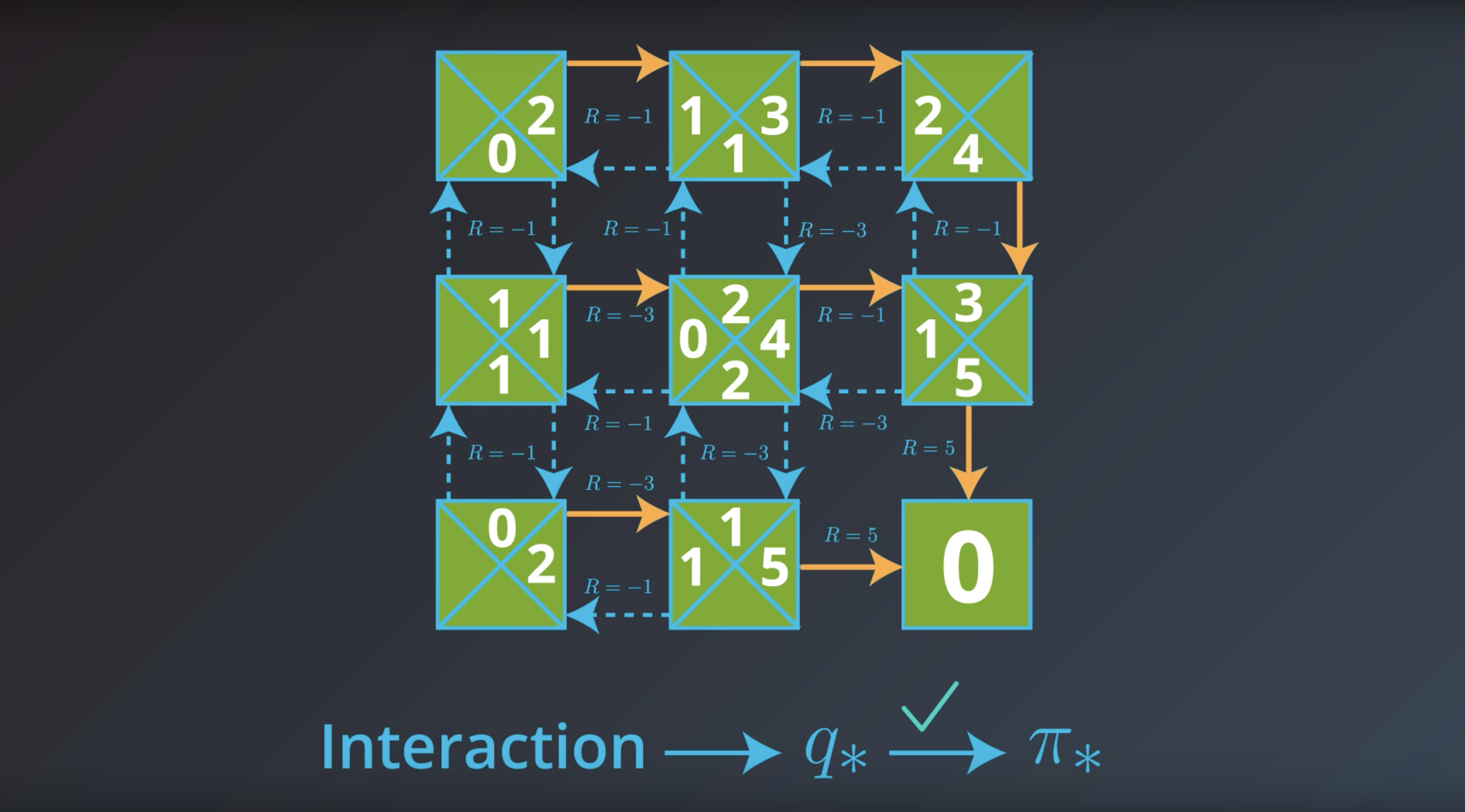
Image(filename='./images/1-2-7-13_if_we_would_have_q_star_then_we_could_get_pi_star.png')

from IPython.display import Image
Image(filename='./images/1-2-7-14_if_we_would_have_pi_star_then_could_We_get_q_star_?.png')

If the agent has optimal value function, it can quickly obtain an optimal policy.

Which is the solution to the MDP that we are looking for.

This is bring us to the question of how the agent could find the optimal value function.

This is in fact…what we’ll study next.

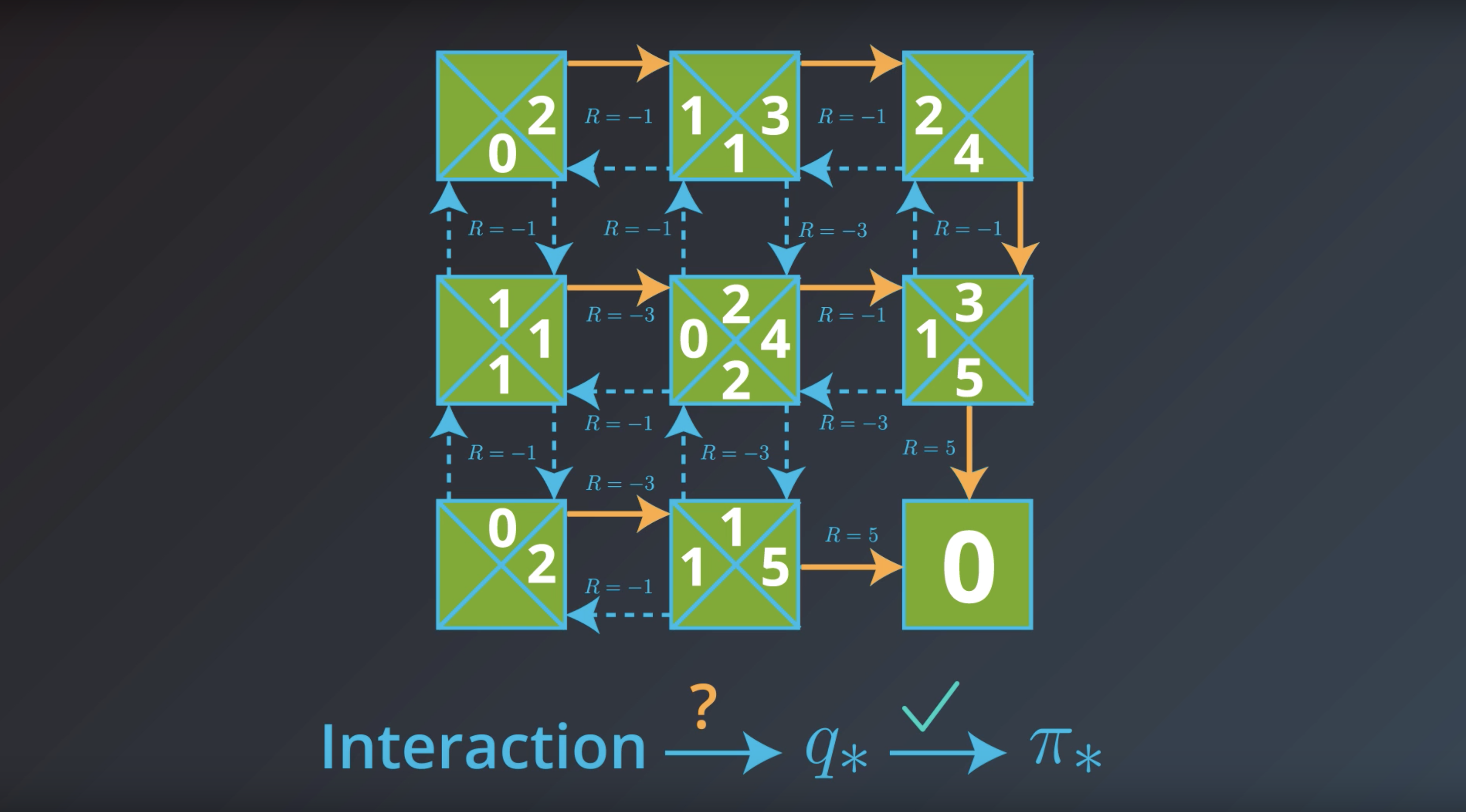
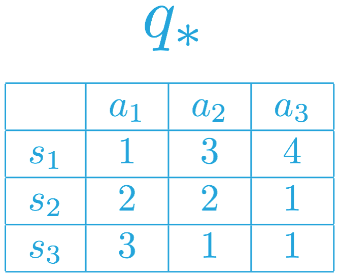
Quiz: Optimal Policies

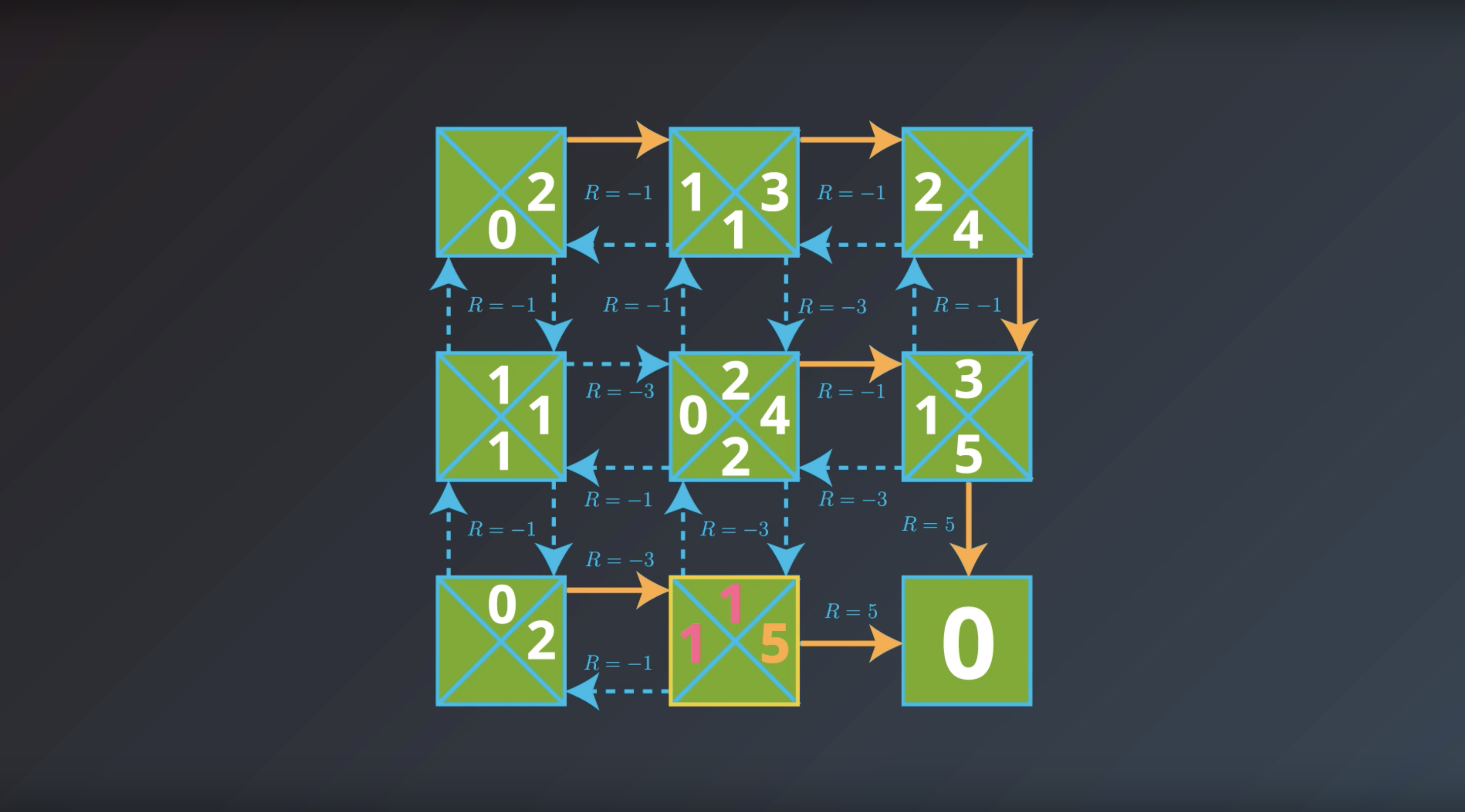
If the state space S and action space A are finite, we can represent the optimal action-value function q∗ in a table, where we have one entry for each possible environment state s∈S and action a∈A.

The value for a particular state-action pair s,a is the expected return if the agent starts in state s, takes action a, and then henceforth follows the optimal policy π∗.

We have populated some values for a hypothetical Markov decision process (MDP) (where S={s1,s2,s3} and A={a1,a2,a3}) below.

from IPython.display import Image
Image(filename='./images/1-2-7-15_Quiz_Optimal_Policies.png')

You learned in the previous concept that once the agent has determined the optimal action-value function q∗, it can quickly obtain an optimal policy π∗ by setting (s)=argmax a∈A(s) q∗(s,a) for all s∈S.

To see why this should be the case, note that it must hold that v∗(s) = max a∈A(s) q∗(s,a).

In the event that there is some state s∈S for which multiple actions a∈A(s) maximize the optimal action-value function, you can construct an optimal policy by placing any amount of probability on any of the (maximizing) actions. You need only ensure that the actions that do not maximize the action-value function (for a particular state) are given 0% probability under the policy.

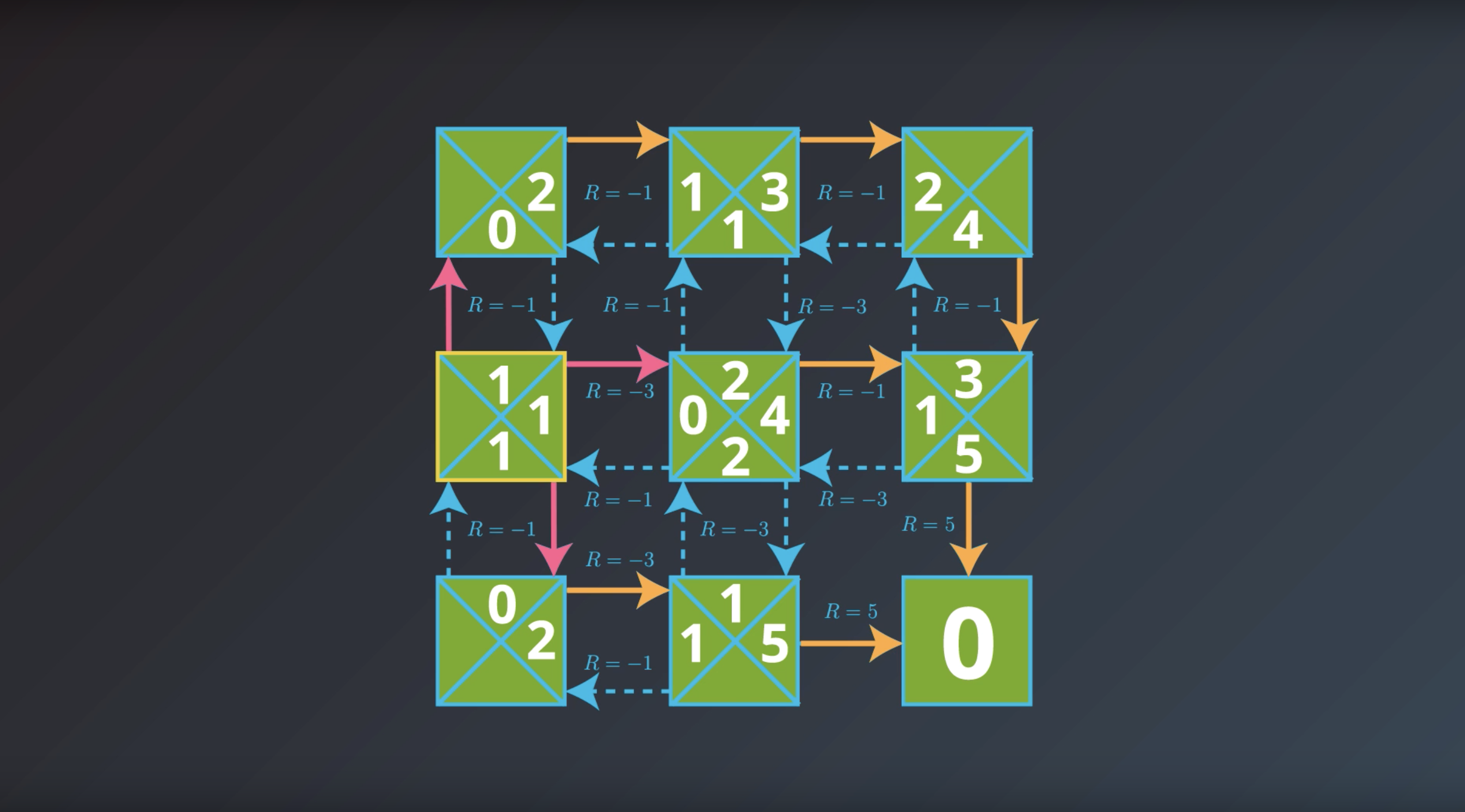
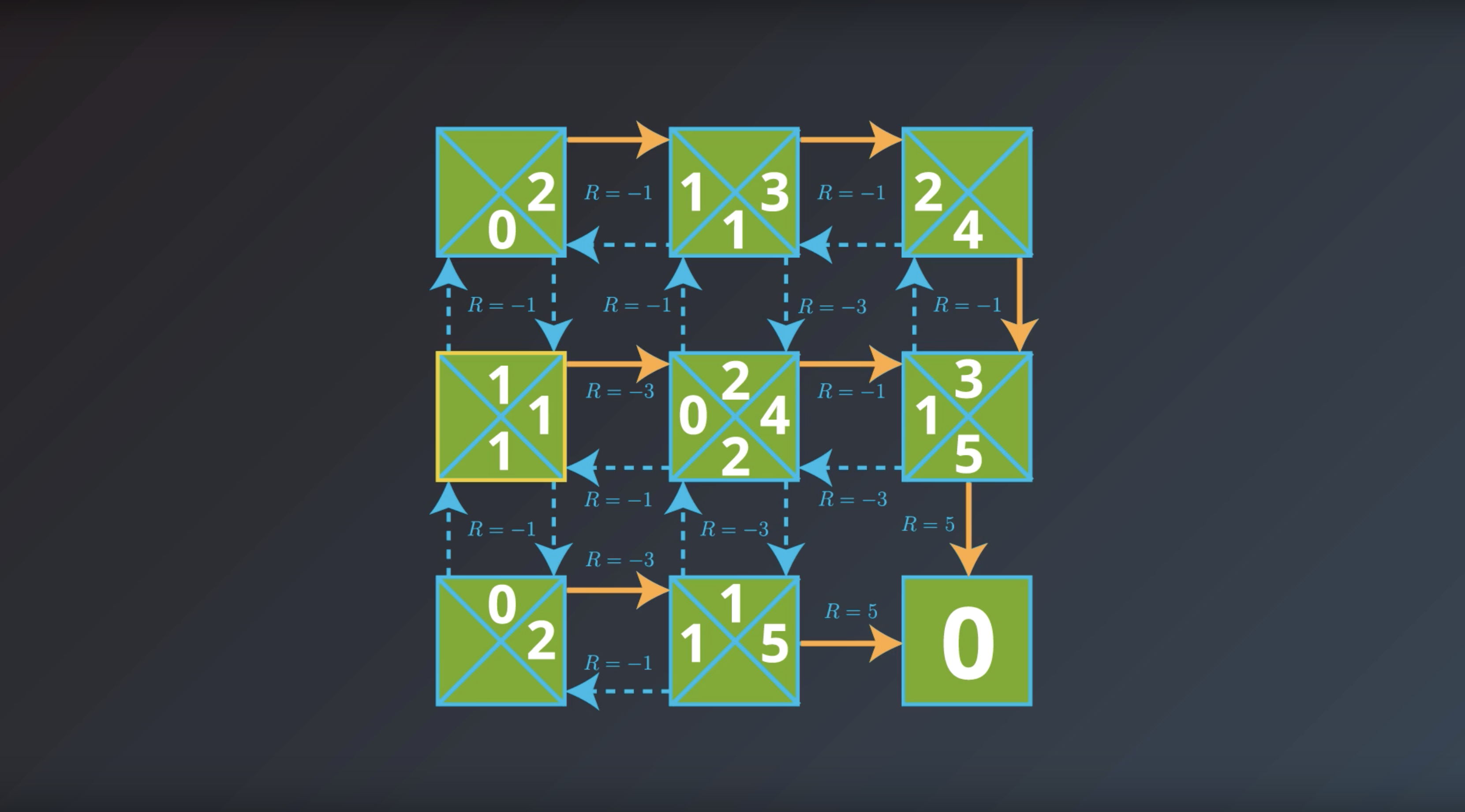
Towards constructing the optimal policy, we can begin by selecting the entries that maximize the action-value function, for each row (or state).

from IPython.display import Image
Image(filename='./images/1-2-7-16_Quiz_Optimal_Policies.png')

Thus, the optimal policy π∗ for the corresponding MDP must satisfy:

• π∗(s1)=a2 (or, equivalently, π∗(a2∣s1)=1), and
• π∗(s2)=a3 (or, equivalently, π∗(a3∣s2)=1).

This is because a2 = argmax a∈A(s1) q∗(s1,a), and a3 = argmax a∈A(s2) q∗(s2,a).

In other words, under the optimal policy, the agent must choose action a2 when in state s1, and it will choose action a3 when in state s2.

As for state s3, note that a1, a2 ∈ argmax a∈A(s3) q∗(s3,a) Thus, the agent can choose either action a1 or a2v under the optimal policy, but it can never choose action a3. That is, the optimal policy π∗ must satisfy:

• π∗(a1∣s3)=p,
• π∗(a2∣s3)=p, and
• π∗(a3∣s3)=0.

where p,q≥0, and p,p+q=1.

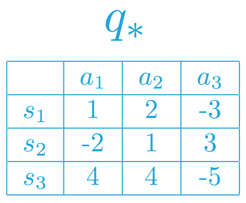
Question 1

Consider a different MDP, with a different corresponding optimal action-value function. Please use this action-value function to answer the following question

from IPython.display import Image
Image(filename='./images/1-2-7-17_Quiz_Optimal_Policies.png')

Which of the following describes a potential optimal policy that corresponds to the optimal action-value function?

1. The agent always selects action a_1 in state s_1.
2. The agent always selects action a_3 in state s_1.
3. The agent is free to select either action a_1 or action a_2 in state s_2.
4. The agent must select action a_3 in state s_2.
5. The agent must select action a_1 in state s_3.
6. The agent is free to select either action a_2 or a_3 in state s_3.