
DRL Actor-Critic Mothods
Updated:
from IPython.display import Image
Image(filename='./images/3-4-0-0_ac_opening.jpg')
Lesson 3-4: Actor-Critic Methods
- Reference book : [“Grokking Deep Reinforcement Learning” by Miguel Morales]{http://bit.ly/gdrl_u}
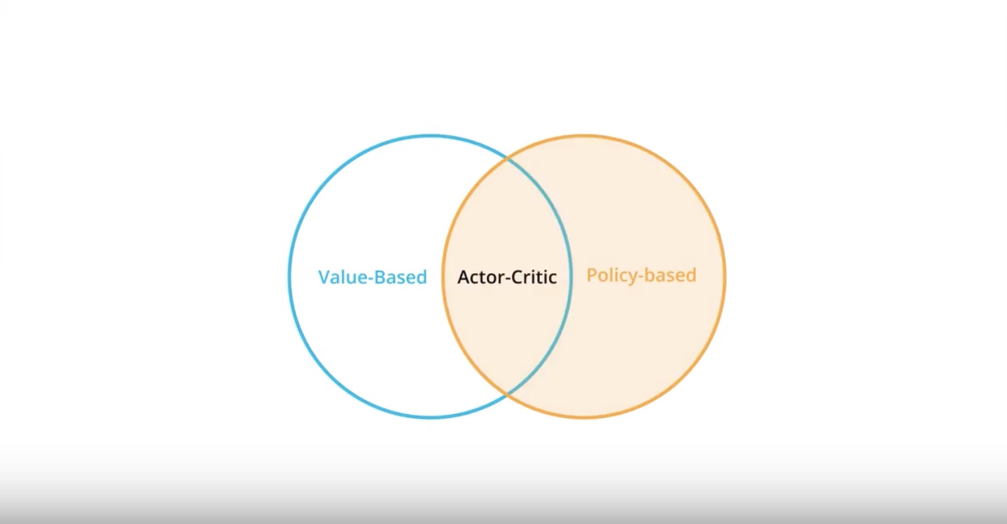
3-4-1 : Actor-Critic Motivation
from IPython.display import Image
Image(filename='./images/3-4-1-1_ac_motivation.jpeg')
from IPython.display import Image
Image(filename='./images/3-4-1-2_ac_value-based_vs_policy-based.jpeg')
from IPython.display import Image
Image(filename='./images/3-4-1-3_ac_stochastic_policy.jpeg')
from IPython.display import Image
Image(filename='./images/3-4-1-4_ac_deterministic_policy.jpeg')
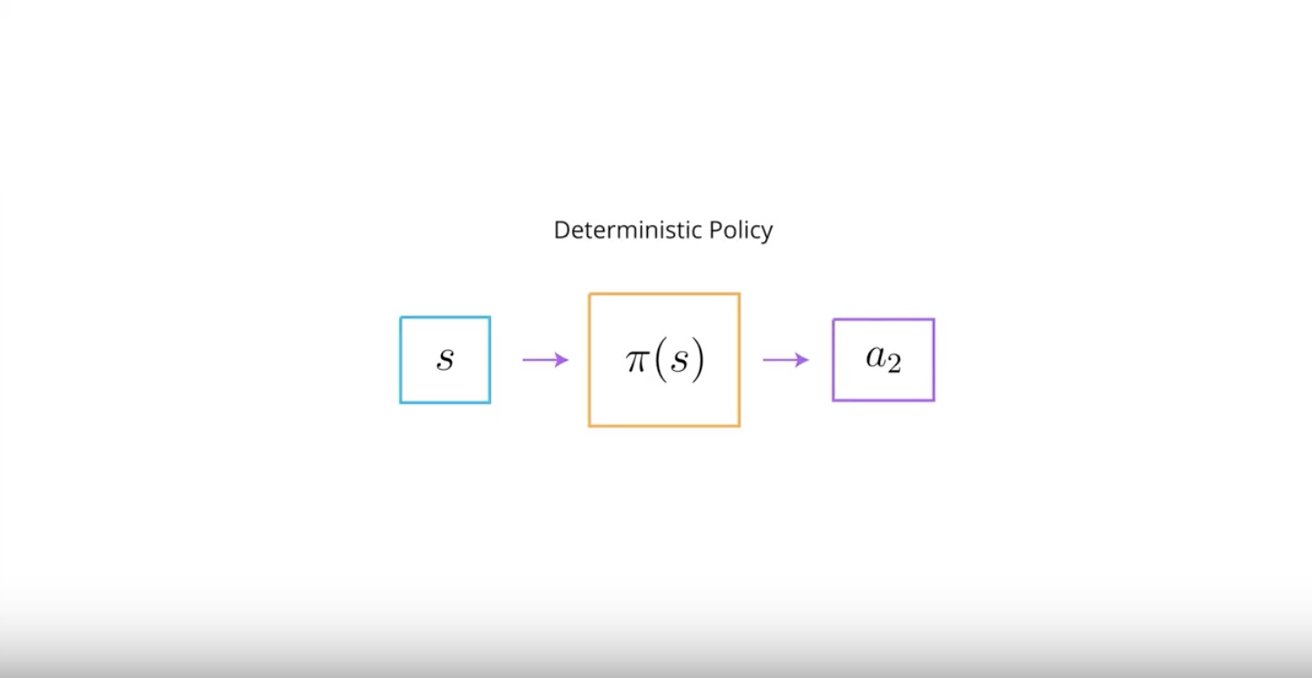
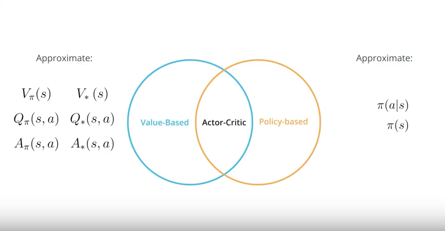
We learn about using baselines to reduce the variance of policy-based method.
We can use a value function as a base.
Think about it if we train a newer network to approximate a value function and use it as a baseline. This baseline further reduce the variance of policy-based methods.
3-4-2 : Bias vs Variance
from IPython.display import Image
Image(filename='./images/3-4-2-1_ac_bias_vs_variance_example.jpeg')

from IPython.display import Image
Image(filename='./images/3-4-2-2_ac_bias_is_high.jpeg')

from IPython.display import Image
Image(filename='./images/3-4-2-3_ac_variance_is_high.jpeg')

from IPython.display import Image
Image(filename='./images/3-4-2-4_ac_bias_vs_variance_quadrant.jpeg')
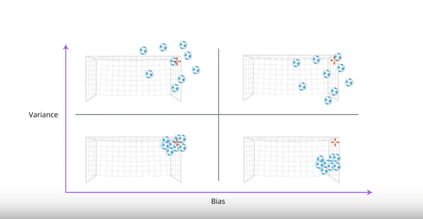
Having both low bias and low varinace is very hard to achieve…
But, now we’ll look at several techniques to be designed to accomplish this…
from IPython.display import Image
Image(filename='./images/3-4-2-5_ac_consider_bias-variance_trade-off.jpeg')
We have to consider the bias-variance trade-off in RL when an agent tries to estimate value functions or polices from returns.
from IPython.display import Image
Image(filename='./images/3-4-2-6_ac_value_function_is_calculated_using_the_expectation_of_returns.jpeg')
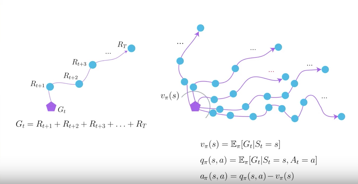
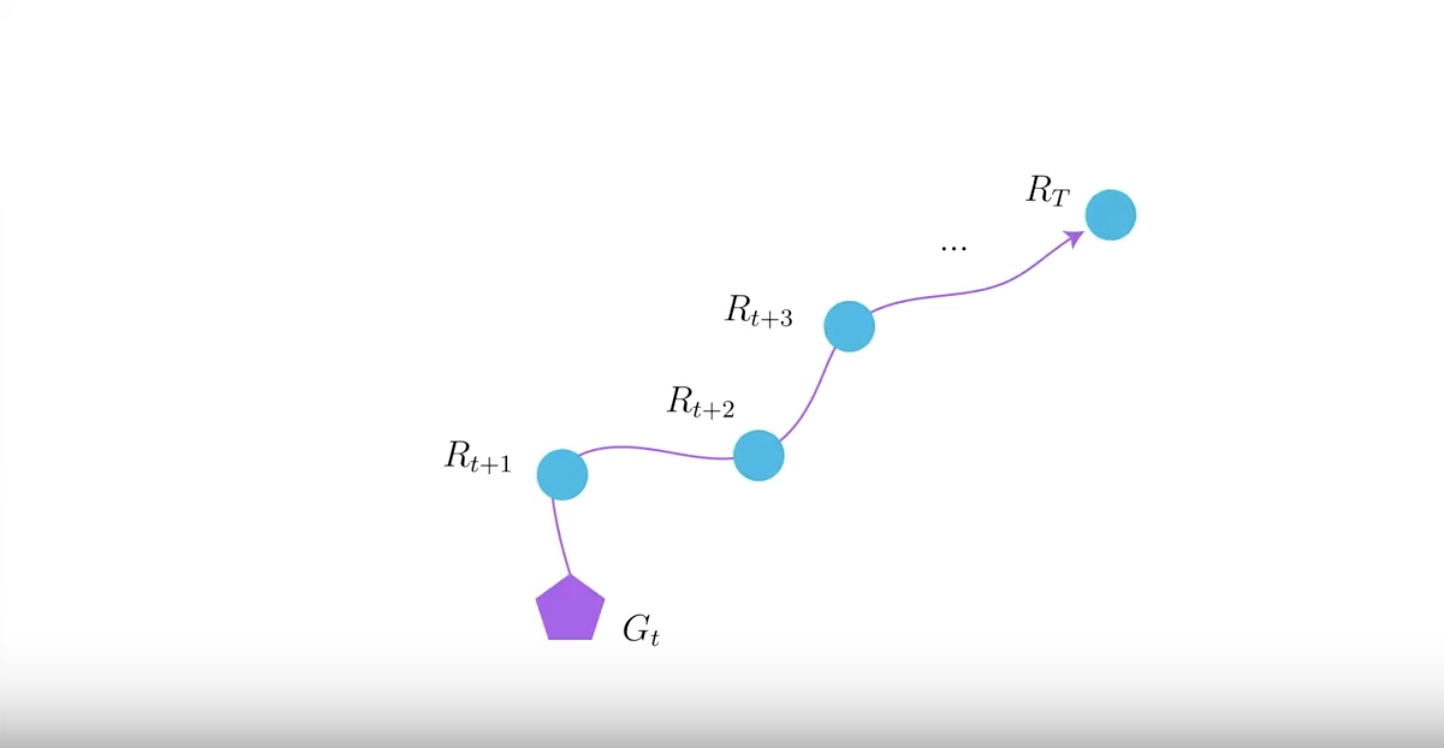
A return is calcurated using a single trajectory. However value functions which we are trying to estimate are calculated using the expectation of returns.
Big part of RL research is an attempt to reduce the variance of algorithms while keeping bias to a minimum
RL agent tries to find policies to maximize the total expected cumulative reward. but since we’re limited to sample in the environment. we can only estimate the expectation.
In Actor-Critic methods…The question is…what is the best way to estimate value functions?
3-4-3 : Two Ways For Estimating Expected Returns
from IPython.display import Image
Image(filename='./images/3-4-3-1_two_ways_estimating_expected_returns.jpeg')
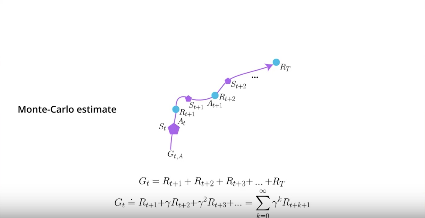
Monte Carlo estimate just adds all the rewards up whether discounted or not.
from IPython.display import Image
Image(filename='./images/3-4-3-2_mc_as_more_as_estimate_we_can_get_better_average_value_function.jpeg')
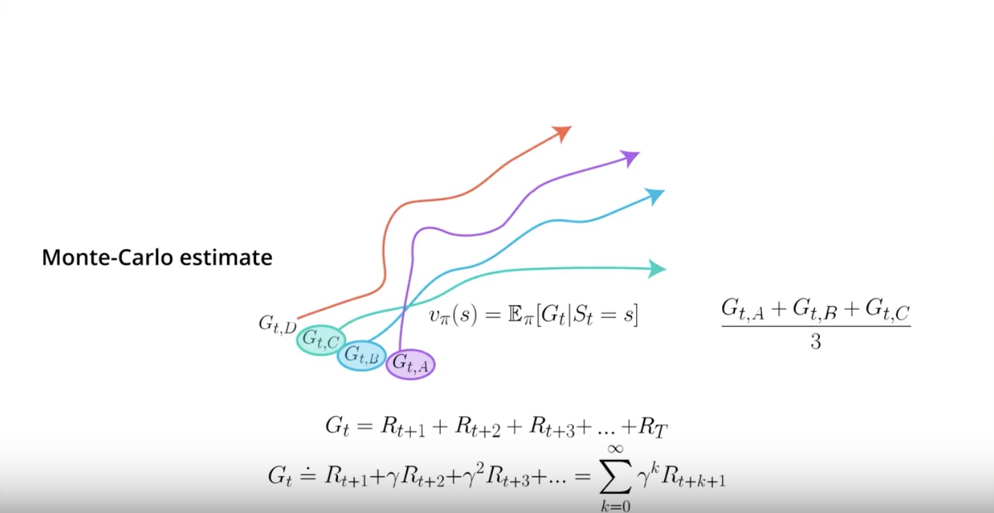
When you have a collection of A, B, C, D, some of those episodes will have trajectories that go through the same states. Each of these episodes can give you a different Monte Carlo estimate for the same value function to calcurate.
All you need to do is average the estimates. Obviously the more estimates you have when taking the average, the better your value function will be.
from IPython.display import Image
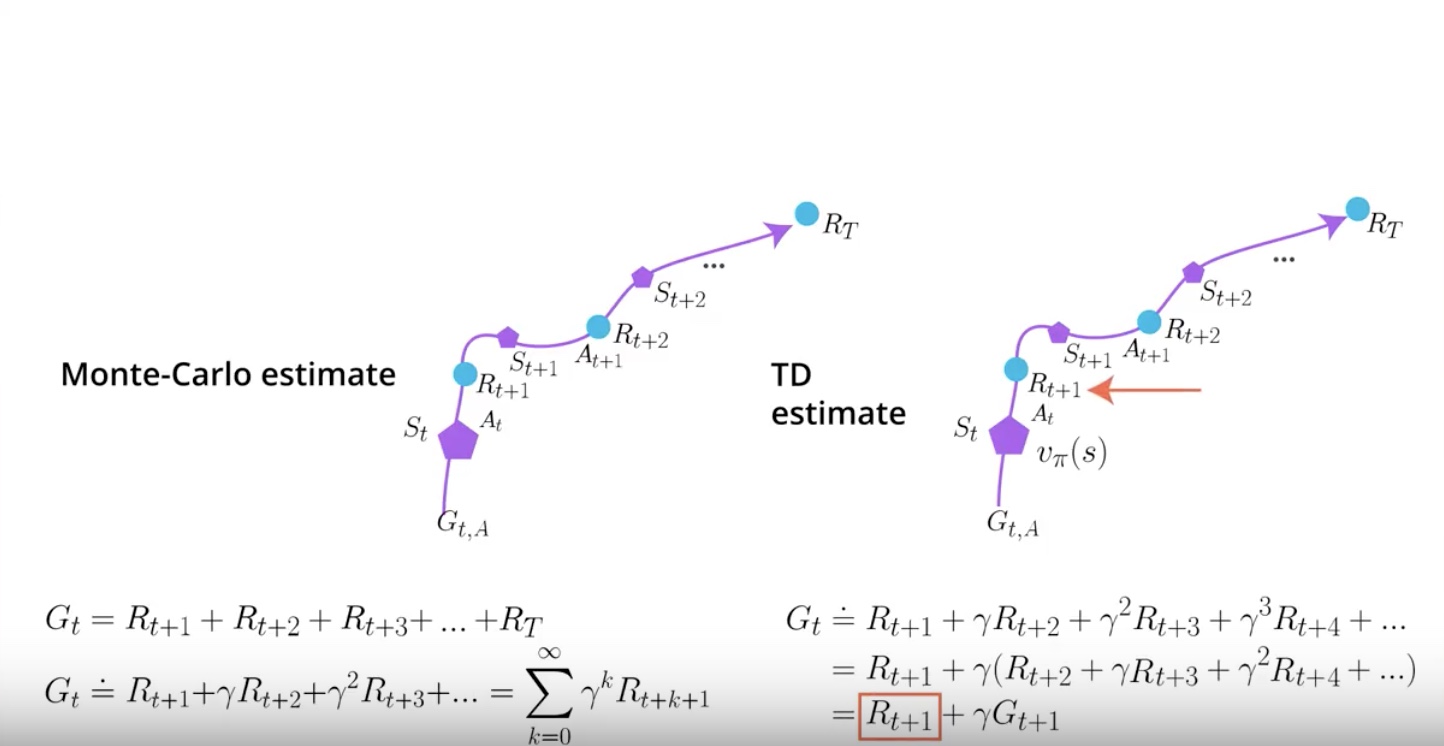
Image(filename='./images/3-4-3-3_td_estimate_current_state-value_using_immediate_reward.jpeg')
from IPython.display import Image
Image(filename='./images/3-4-3-4_td_and_an_estimate_of_the_discounted_return_from_next_state.jpeg')
from IPython.display import Image
Image(filename='./images/3-4-3-5_td_need_next_state_tvalue-function_to_calcurate_current_state_value-function.jpeg')
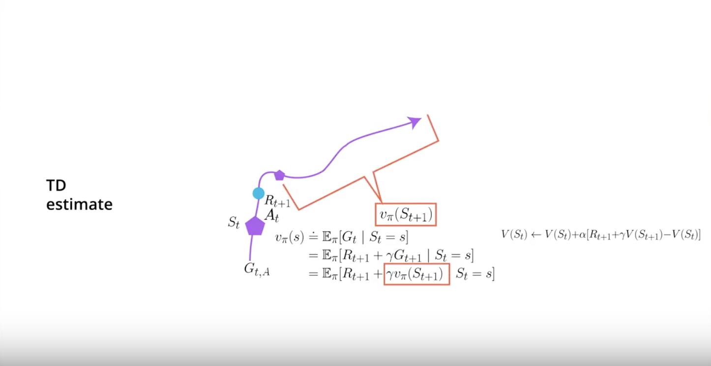
In Temporal Difference, you start in the state ‘St’, take action ‘At’ at the environment. then transition gives you reward ‘Rt+1’ and send you to a new state ‘St+1’.
But then you can actually stop there by the magic of ‘Dynamic Programming’. it also called by ‘Bootstrapping’.
from IPython.display import Image
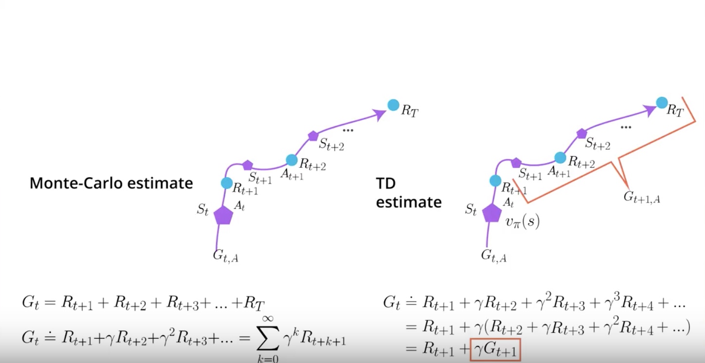
Image(filename='./images/3-4-3-6_td_calcurate_a_new_estimate_for_current_state_by_dynamic_programming.jpeg')
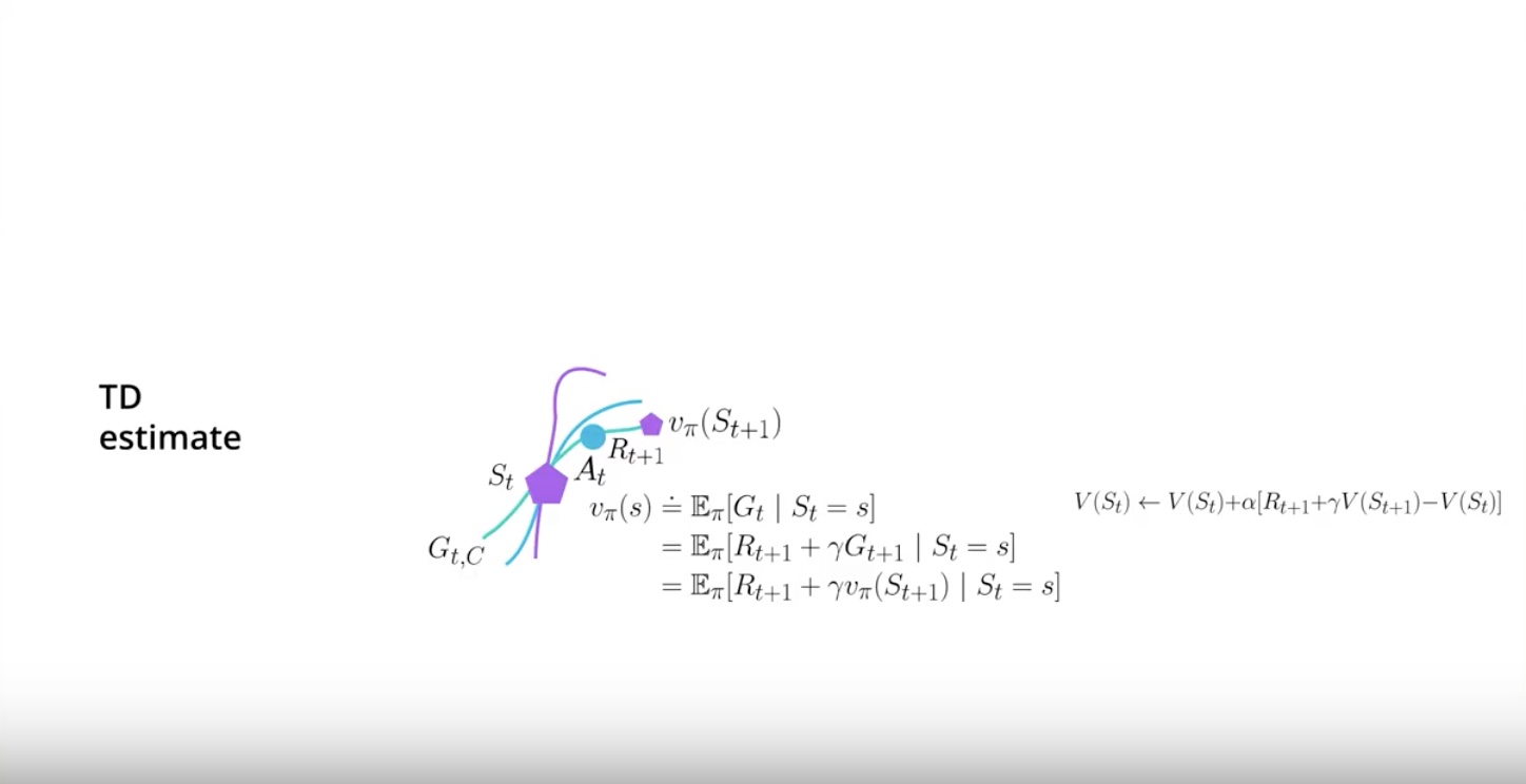
‘Dynamic Programming (= Bootstrapping)’ means that you can leverage the estimate that you currently have for the next state in order to calcurate a new estimate for the value function of the current state.
Now the estimates of the next state will probably be off particularlly early on. But that value will become better and better as you have more data.
More data makes other values better.
from IPython.display import Image
Image(filename='./images/3-4-3-7_mc_high-variance_low_bias_why.jpeg')
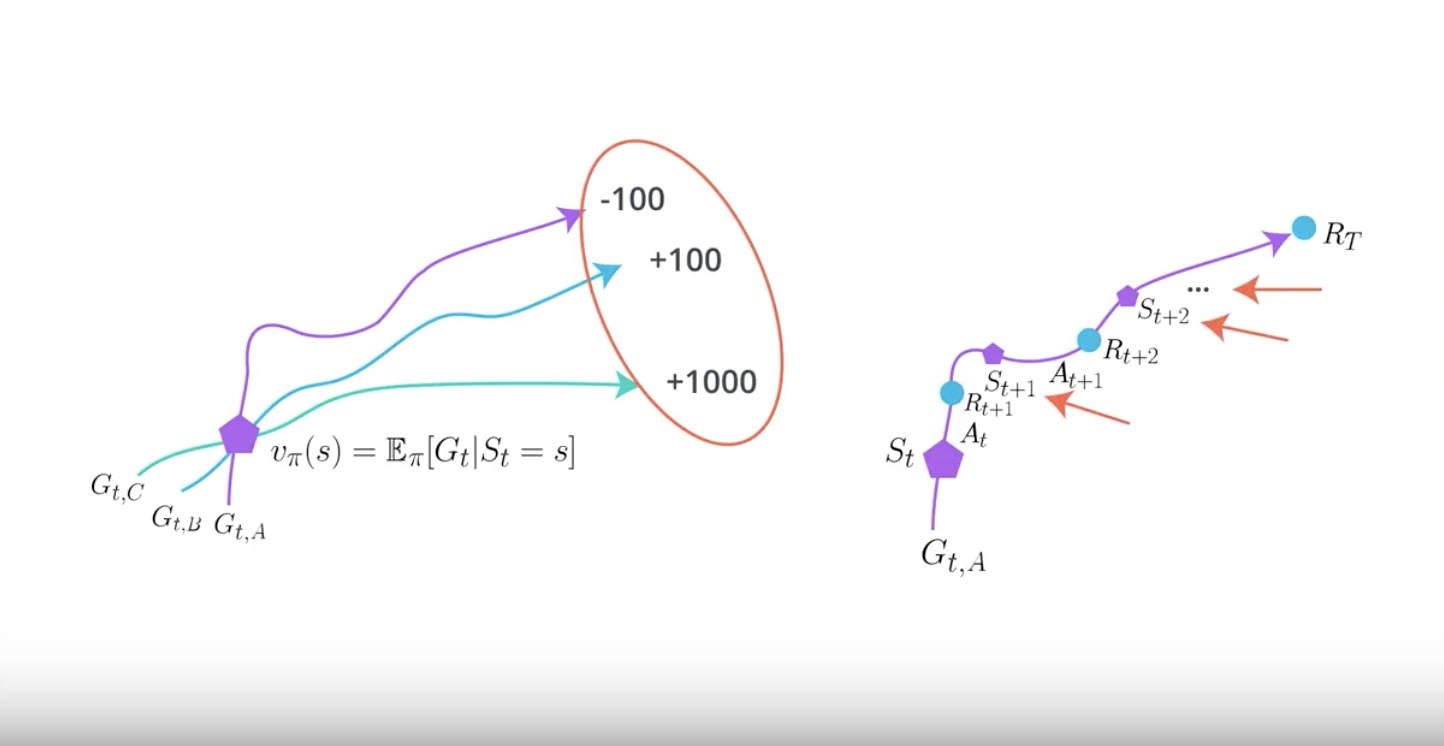
Why is Monte Carlo estimates will have High-Varinace?
- Because you are compounding lots of random events that happen during the course of a single episode.
Why is Monte Carlo estimates will have Low-Bias ?
- Because you are using the true rewards you obtained. so given lots of date you estimate will be accurate.
from IPython.display import Image
Image(filename='./images/3-4-3-8_tc_low-variance_high_bias_why.jpeg')
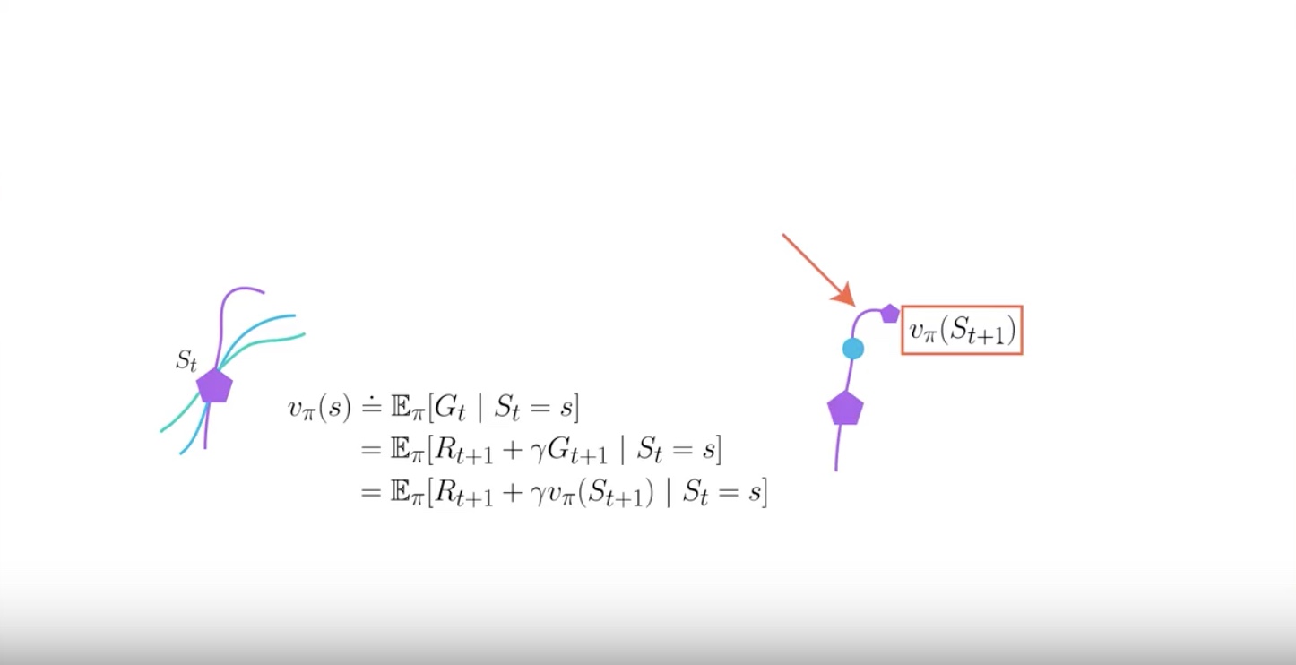
Why is Temporal Difference estimates will have Low-Varinace?
- Because you are only compounding a single time step of randomness instead of a full rollout.
Why is Temporal Difference estimates will have High-Bias ?
- Because you are bootstrapping on the next state estimates and those are not true values so you are adding bias into your calcuration.
Finally your agent will learn faster but will have more problems converging.
3-4-4 : Policy-based, Value-based and Actor-Critic
from IPython.display import Image
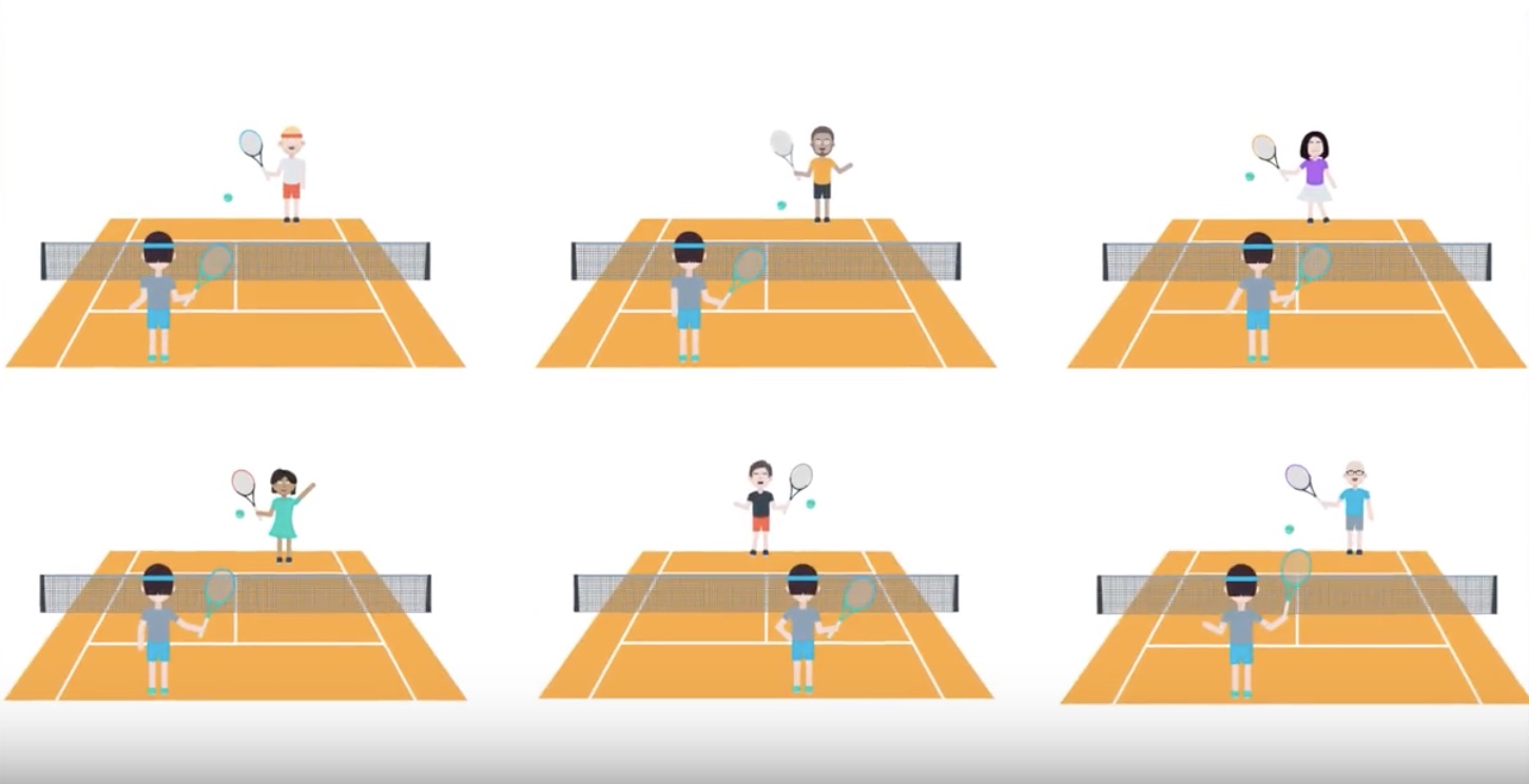
Image(filename='./images/3-4-4-1_pb_vb_ac_intuition_learning_how_to_play_tennis.jpeg')
from IPython.display import Image
Image(filename='./images/3-4-4-2_policy-based_method_example.jpeg')

from IPython.display import Image
Image(filename='./images/3-4-4-3_value-based_method_example.jpeg')

from IPython.display import Image
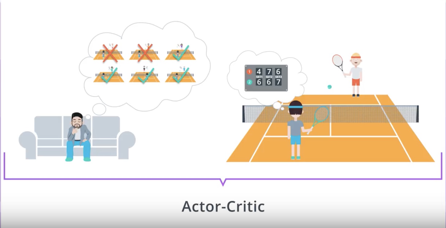
Image(filename='./images/3-4-4-4_actor-critic_method_example.jpeg')
3-4-5 : A Basic Actor-Critic Agent
Actor-Critic agent is an agent that uses Function Approximation to learn a policy and a value function.
And we will use tuner networks. One for Actor and one for Critic.
The Critic learn to evaluate the State-Value function Vπ using TD estimate.
When we use the Critic, we will calcurate the Advantage function and train the Actor using this value
from IPython.display import Image
Image(filename='./images/3-4-5-1_ac_basic_online_actor-critic_have_two_networks.jpeg')
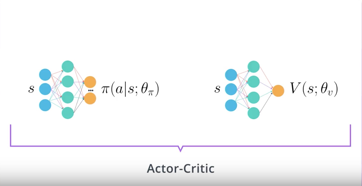
Actor network takes in a state and outputs distribution of actions.
Critic network takes in a state and outputs a state-value function of policy Vπ.
from IPython.display import Image
Image(filename='./images/3-4-5-2_ac_actor-critic_algorithm_1st_step.jpeg')
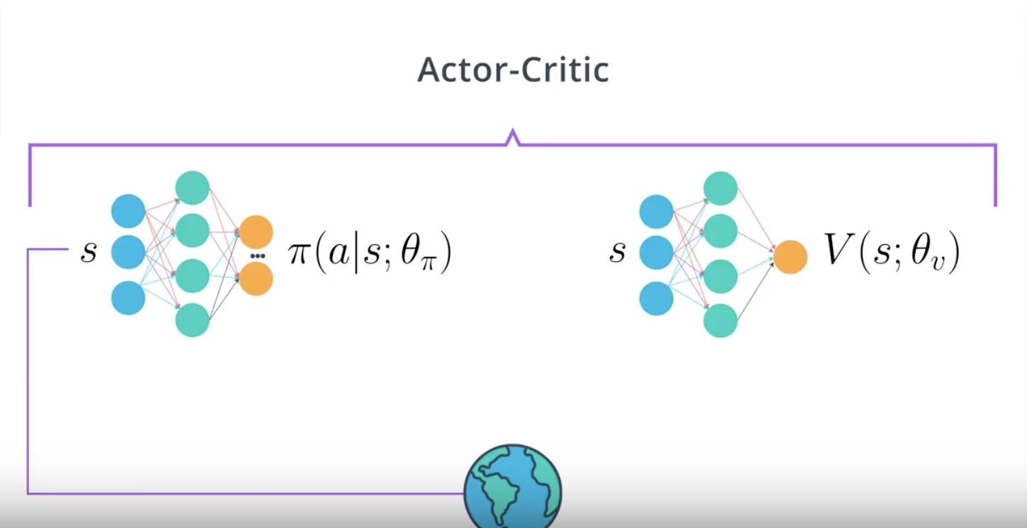
1st step : Input current state into the actor network
from IPython.display import Image
Image(filename='./images/3-4-5-3_ac_actor-critic_algorithm_2nd_step.jpeg')

2nd step : Get the action to take in the current state and observe next state and reward
from IPython.display import Image
Image(filename='./images/3-4-5-4_ac_actor-critic_algorithm_3rd_step.jpeg')
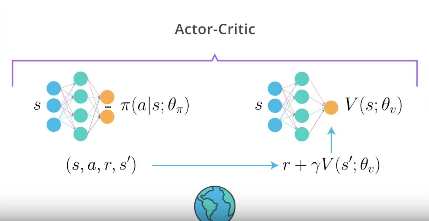
3rd step : Using the TD estimate which is the reward r plus value estimate for s prime gamma times, so r plus gamma times V of s prime.
from IPython.display import Image
Image(filename='./images/3-4-5-5_ac_actor-critic_algorithm_4th_step.jpeg')
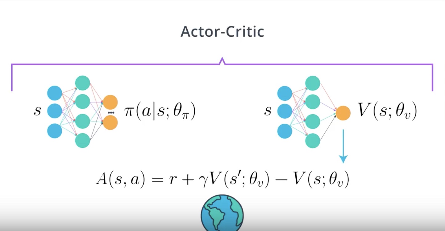
4th step : Train Critic and calcurate Advantage function
from IPython.display import Image
Image(filename='./images/3-4-5-6_ac_actor-critic_algorithm_5th_step.jpeg')
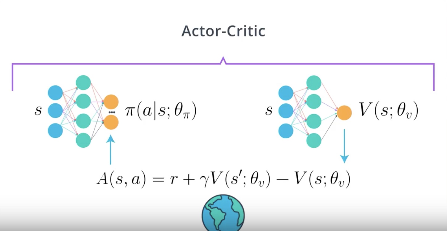
5th step : Train Actor using the calcurated Advantage Fuction as a baseline
Notation
- V(s;θ) or A(s,a) = oversimplification of Vπ(s;θ) or Aπ(s,a)
- A∗(s,a) = optimal advantage function
- θv = such value function is using a neural network. For example, V(s;θ) is using a neural network as a function approximator. , but A(s,a) is not. We are calculating the advantage function A(s,a) using the state-value function V(s;θ), but A(s,a) is not using function approximation directly.
3-4-6 : A3C: Asynchronous Advantage Actor-Critic, N-step Bootstrapping
A3C calcurate Advantage function, Aπ(s,a) and the Critic will be learning to estimate Vπ(s;θ).
If we use images as input, A3C use CNN with Actor and Critic sharing weights to two seperate heads. one for the Actor and one for the Critic.
A3C is not to be used exclusively with CNN and images but if you were to use it, Sharing weights is more efficient…but more complexed and harder to train.
It’s good idea to start with two networks and change it only to improve performance.
One interesting aspect of A3C is using N-step Bootstrapping instead of using TD estimate.
from IPython.display import Image
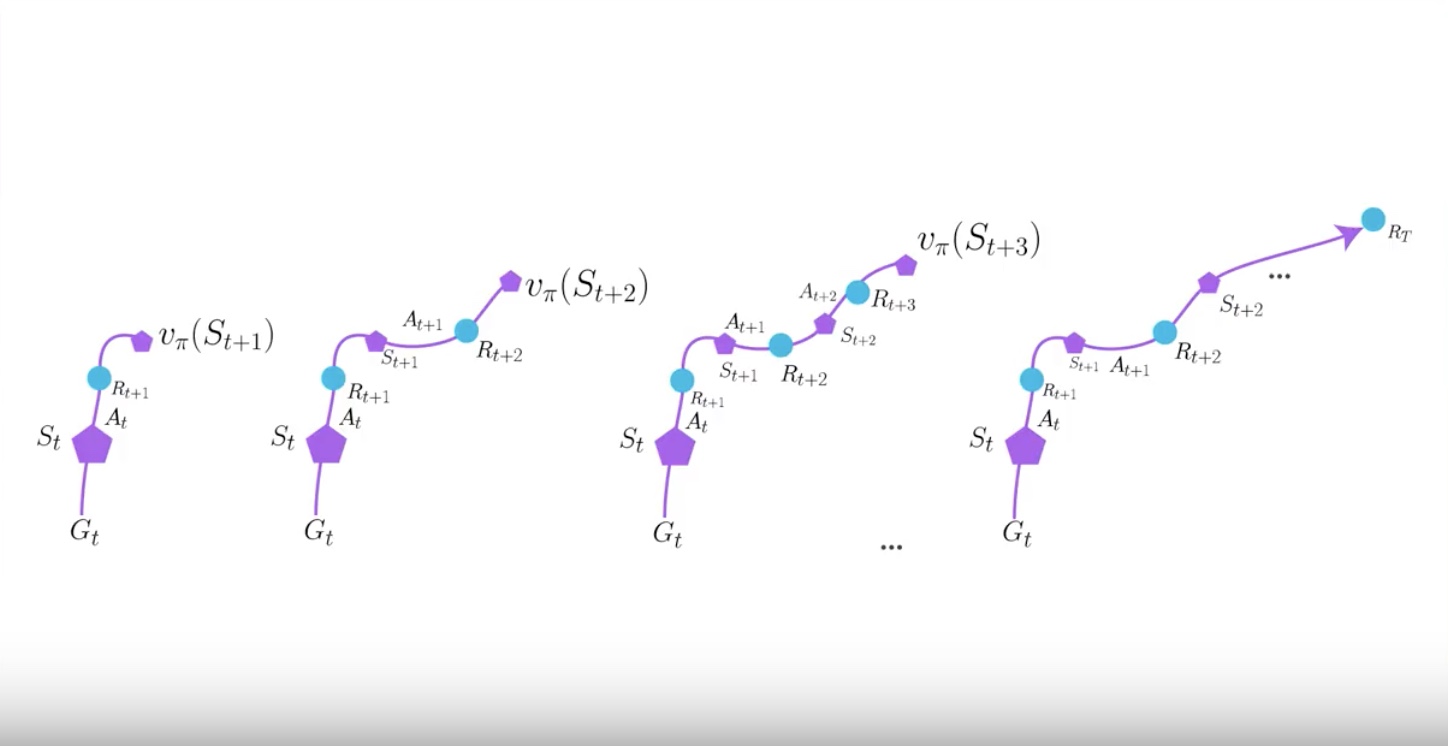
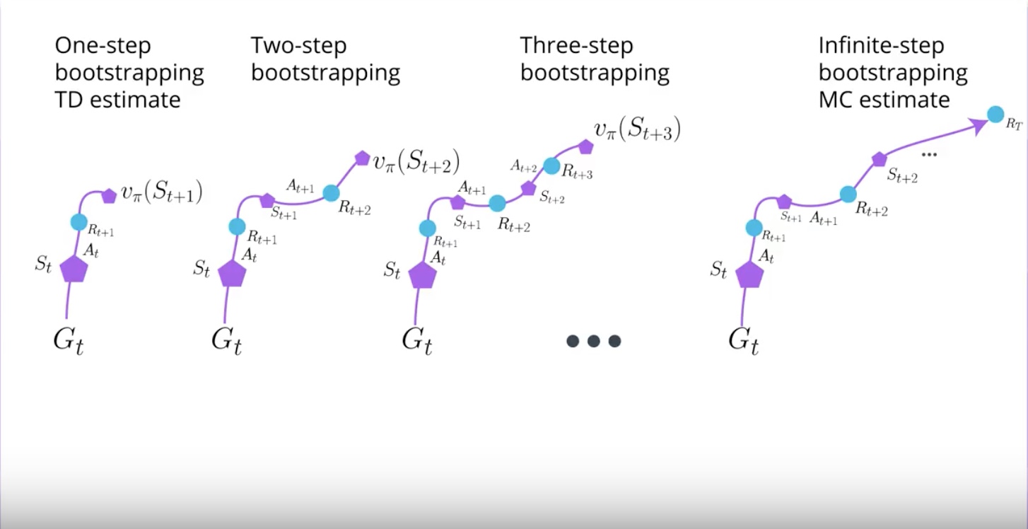
Image(filename='./images/3-4-6-1_a3c_n-step_bootstrapping.jpeg')
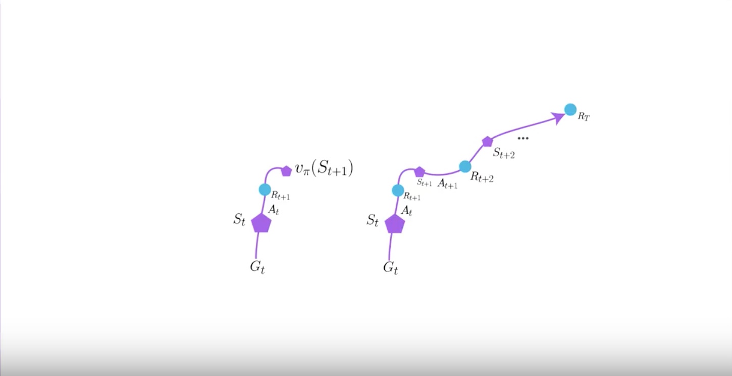
N-step Bootstrapping is just an abstraction and a generalization of TD and Monte Carlo estimate.
TD is an 1-step Bootstrapping. your agent experince one time step of real reward and bootstrap right there.
Monte Carlo goes out all the way and does not bootstrap. Monte Carlo is infinite-step Bootstrapping.
from IPython.display import Image
Image(filename='./images/3-4-6-2_a3c_n-step_bootstrapping_example.jpeg')
How about going more than 1-step? Can we do 2 time steps of real reward and bootstrap the second next state? Can we do 3 time steps or 4, 5, and so on?
This approach looks like waiting to experience the environment for a little longer before you calcurate the expected return of the original state. It allows you to have less bias in your prediction keeping variance on the control.
Only 4 or 5-step Bootstrapping are often the best.
By using N-step Bootstrapping, A3C propagates values to the last end state, which allows you to have faster convergence with less experience required while still keeping variance on the control.
3-4-7 : A3C: Asynchronous Advantage Actor-Critic, Parallel Training
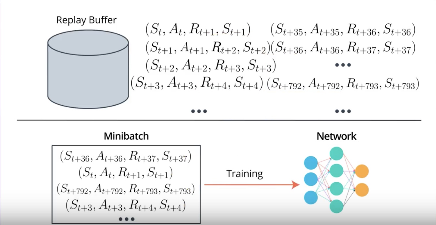
- Unlike DQN A3C doesn’t use the Replay Buffer. The main reason we needed Replay Buffer was…so that we could corelate experience.
from IPython.display import Image
Image(filename='./images/3-4-7-1_a3c_parallel_training.jpeg')
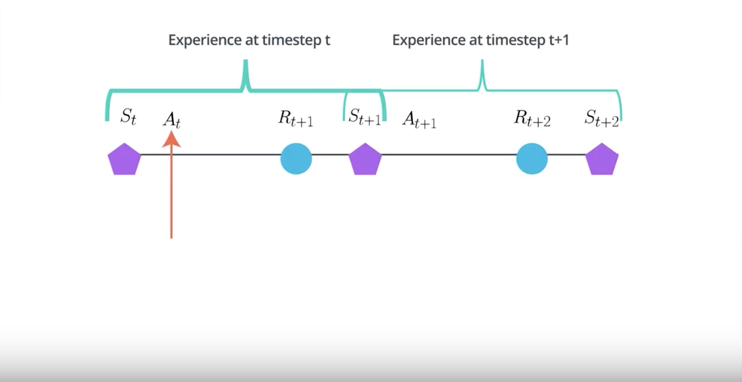
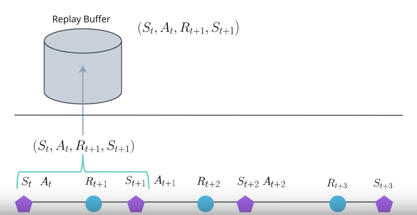
In RL, the agent collects experience in a sequential manner.
The experience at the time step T+1 will be correlated to the experience at the time step T.
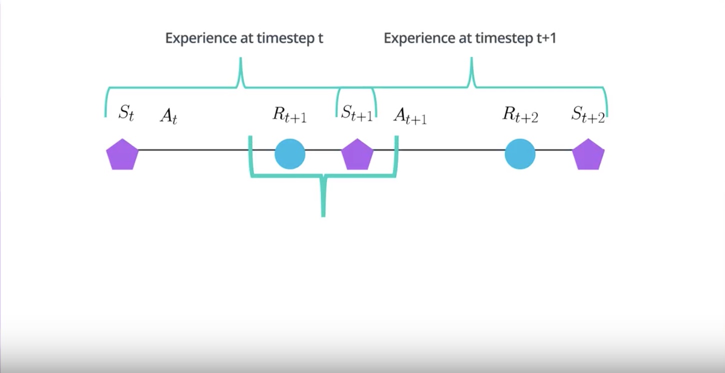
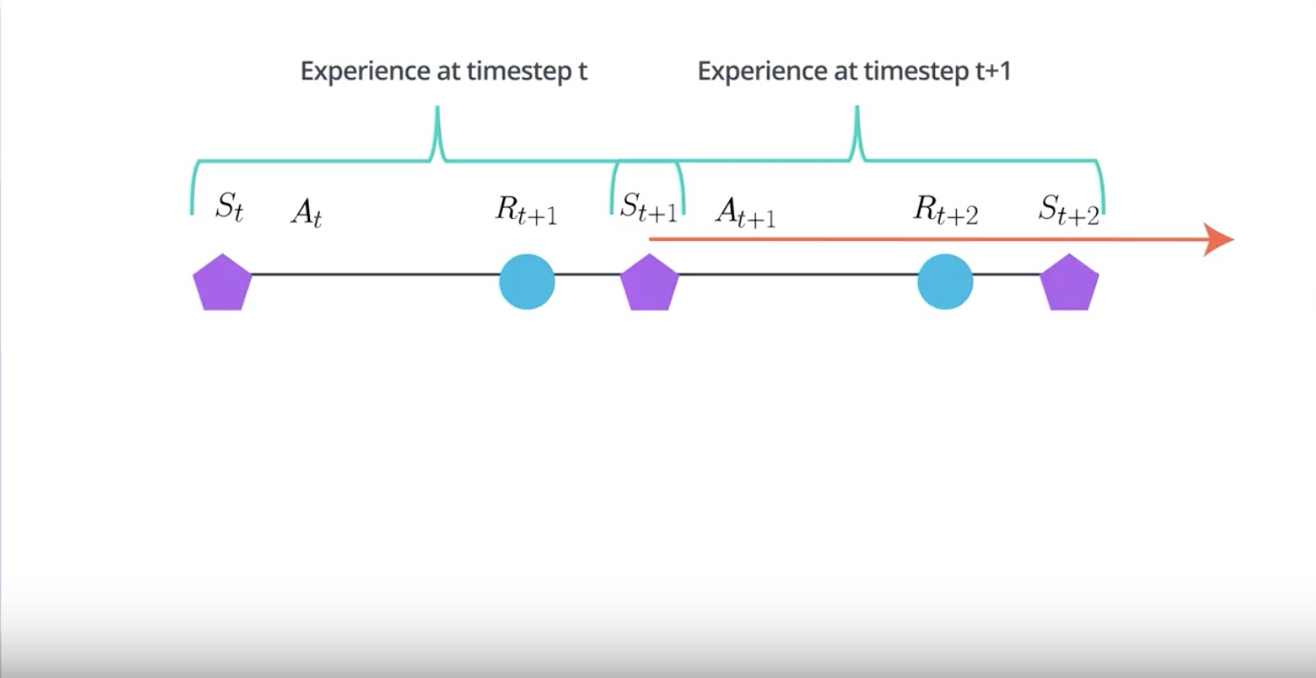
Because it is action taken at the time step T that is partially responsible for the reward and the state observed at the time step T+1.
from IPython.display import Image
Image(filename='./images/3-4-7-2_a3c_parallel_training_explain.jpeg')
from IPython.display import Image
Image(filename='./images/3-4-7-3_a3c_parallel_training_observed_state_influence_the_future_dicision.jpeg')
from IPython.display import Image
Image(filename='./images/3-4-7-4_a3c_replay_buffer_1st_step.jpeg')
from IPython.display import Image
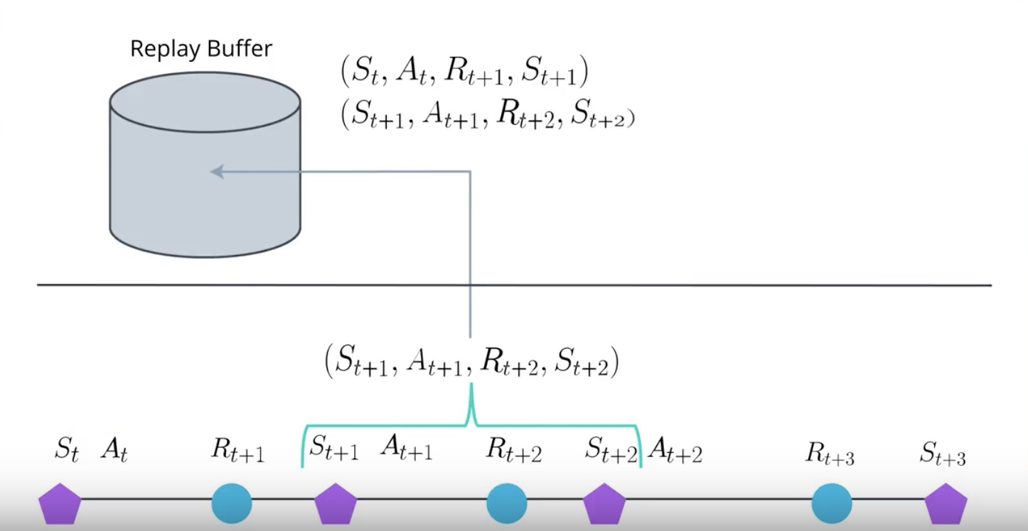
Image(filename='./images/3-4-7-5_a3c_replay_buffer_2nd_step.jpeg')
from IPython.display import Image
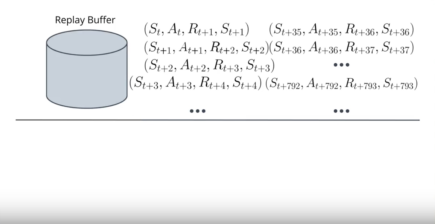
Image(filename='./images/3-4-7-6_a3c_replay_buffer_3rd_step.jpeg')
from IPython.display import Image
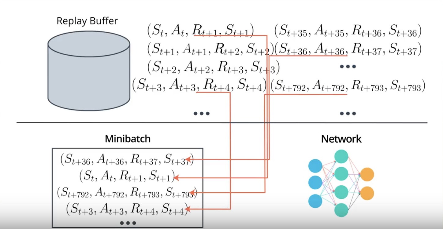
Image(filename='./images/3-4-7-7_a3c_replay_buffer_4th_step.jpeg')
from IPython.display import Image
Image(filename='./images/3-4-7-8_a3c_replay_buffer_5th_step.jpeg')
from IPython.display import Image
Image(filename='./images/3-4-7-9_a3c_replace_rb_with_parallel_training_by_creating_multiple_instances.jpeg')
from IPython.display import Image
Image(filename='./images/3-4-7-10_a3c_samples_will_be_decorrelated_because_agents_will_likely_be_experienced_in_different_states.jpeg')
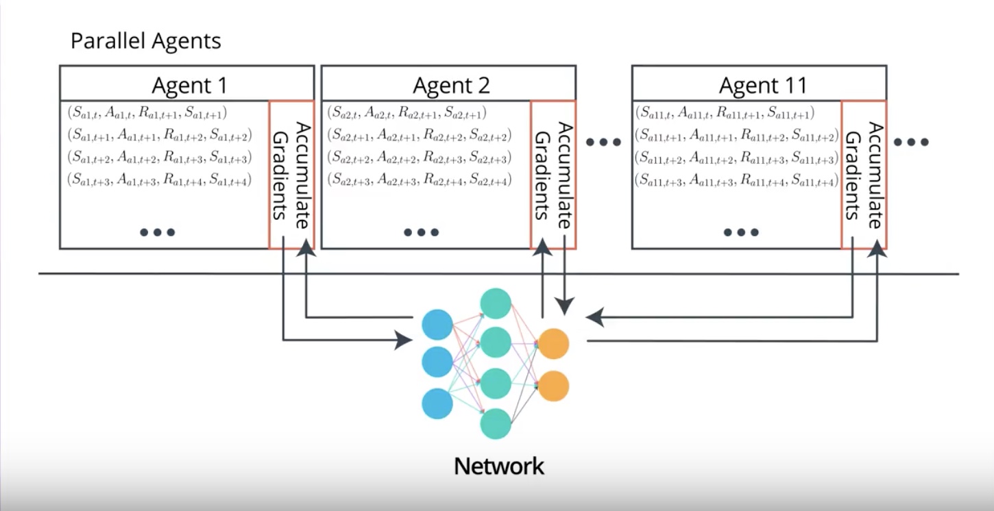
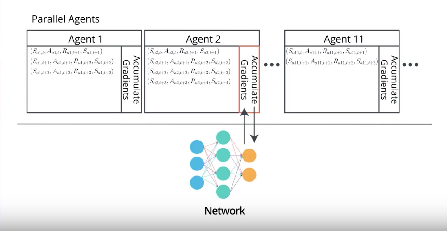
A3C replaces Replay Buffer with parallel training by creating multiple instances of the environment and the agent. and runs them at the same time.
Each agent will receive many batches of the correlated experiences. but samples will be decorrelated because agents will likely be experienced in different states at any given time.
This way of training allows us On-Policy learning which is often associated with more stable learning.
3-4-8 : A3C: Asynchronous Advantage Actor-Critic, Off-policy vs. On-policy
On-Policy learning is… “when policy is used for interacting with the environment is also the policy being learn”.
Off-Policy learning is… “when policy is used for interacting with the environment is different than the policy being learn”.
SARCA is a good example of On-Policy learning.
Q-Learning is a good example of Off-Policy learning.
from IPython.display import Image
Image(filename='./images/3-4-8-1_a3c_on-policy_sarsa.jpeg')
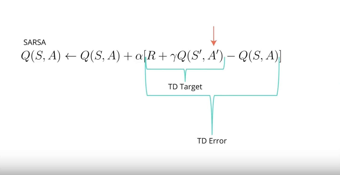
In SARSA, the action used for calcurating the TD target, and the TD error is the action that the agent will take in the following time step A prime.
from IPython.display import Image
Image(filename='./images/3-4-8-2_a3c_off-policy_q-learning.jpeg')
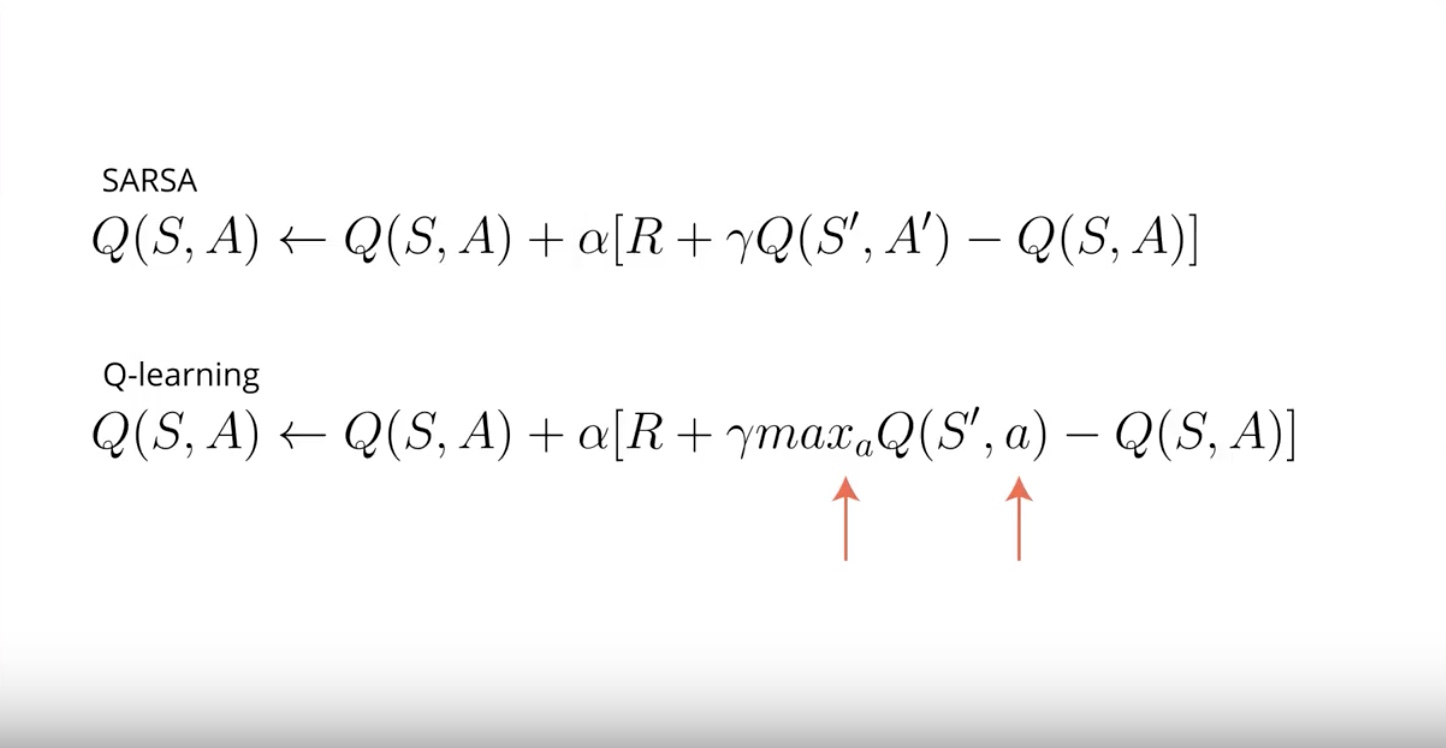
In Q-Learning, the action used for calcurationg the target , the action with the highest value. but this action is not guaranteed to be used by the agent for interacting with the environment in the following step.
In Q-Learning, A prime is note necessary.
Q-Learning learns the deterministic optimal policy even if its behavior is totally random.
SARSA learns the best exploratory policy that is the best policy that still explores
Off-Policy learning
- DQN is an Off-Policy learning.
- Off-Policy learning is known to be unstable and often diverse with neural networks.
On-Policy learning
- A3C is an On-Policy learning.
- In On-Policy learning, you only use the data generated by policy currently being learned about. and anytime you improve your policy you toss out all data and go out collect some more on.
- On-Policy learning is a bit inefficient in the use of experiences but it often has more stable and consistent convergence.
Optional Reference about On/Off Policy learning
“Q-Prop: Sample-Efficient Policy Gradient with An Off-Policy Critic” by Shixiang Gu, Timothy Lillicrap, Zoubin Ghahramani, Richard E. Turner, Sergey Levine (Submitted on 7 Nov 2016 (v1), last revised 27 Feb 2017 (this version, v3))
Link to the Q-Prop paper by Google : https://arxiv.org/abs/1611.02247
3-4-9 : A2C: Advantage Actor-Critic
from IPython.display import Image
Image(filename='./images/3-4-9-1_a2c_has_synchronization_point.jpeg')
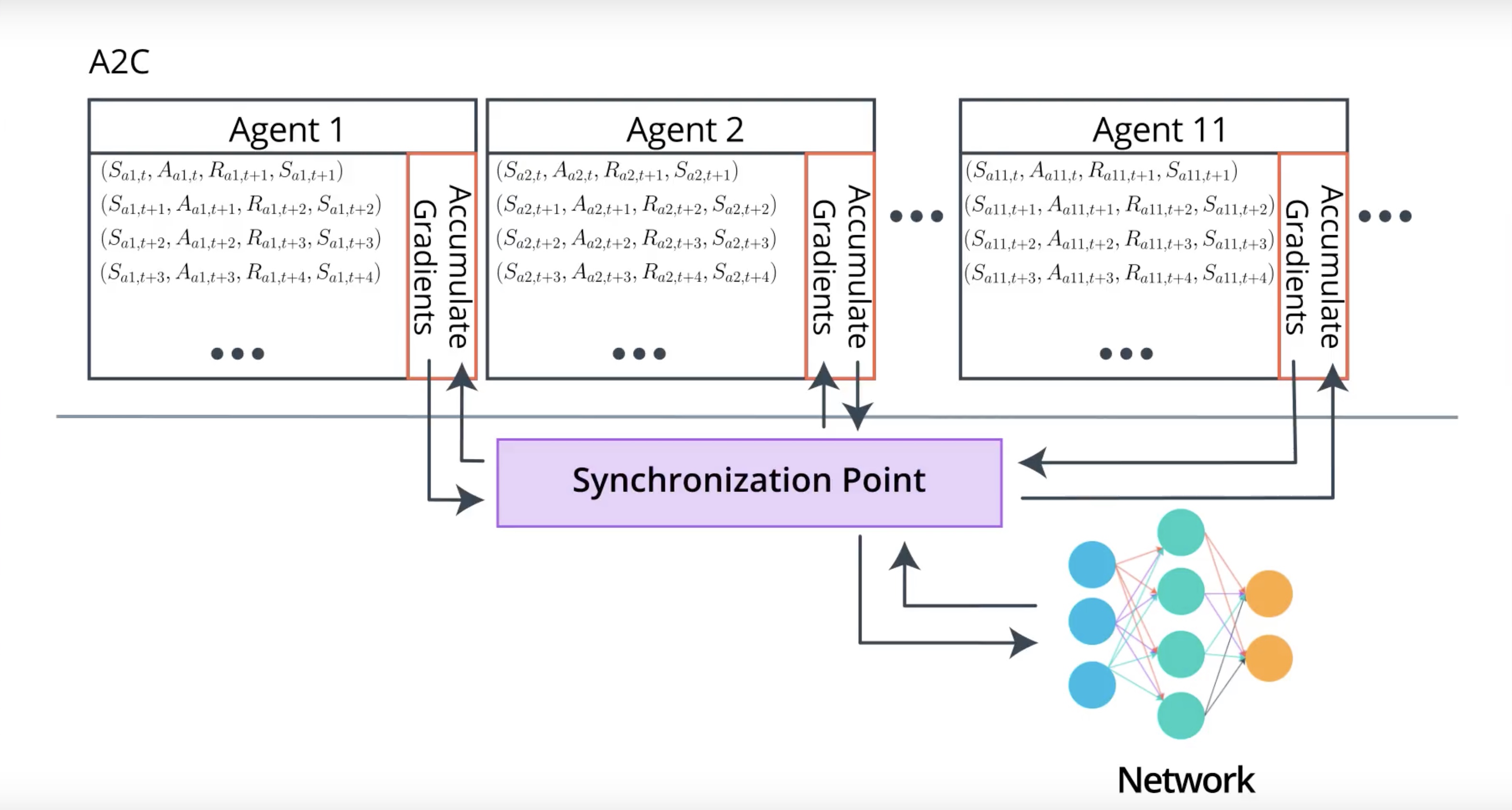
In A3C, each agents update network on its own. but there is no synchronization between the agents. It means that the weights an agent using might be different from the weights in use by the another agent.
In A2C, there is an extra code that synchronize all agents. It waits for all agents to finish a segment of interaction with its copy of the environment then update the network at once and then send updated weights back to the agents.
A2c has simpler architecture but has almost same results with A3C. some cacse are better than A3C
A3C is most easily trained on a CPU. A2C is more straightfoward to extend to a GPU implementation.
3-4-10 : GAE: Generalized Advantage Estimation
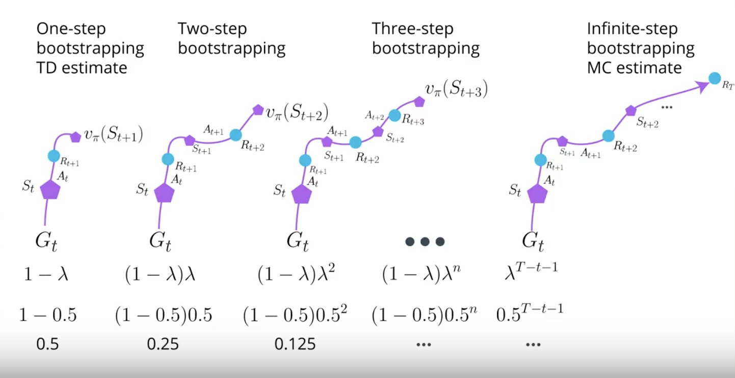
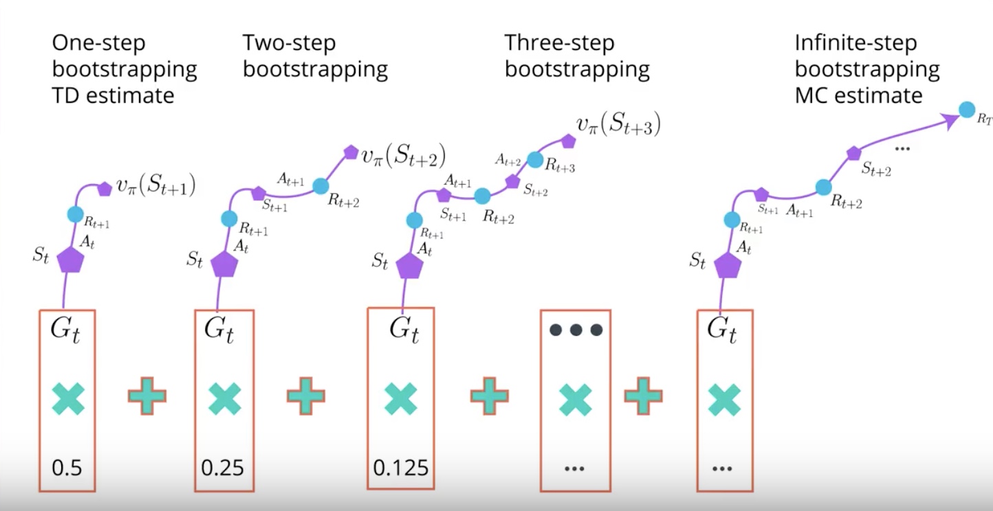
There is another way for estimating expected return called the lamda return.
from IPython.display import Image
Image(filename='./images/3-4-10-1_gae_which_is_the_better_n_mumber.jpeg')
When you try N-step Bootstrapping, you realize that number of N larger than one often performs better. but still hard to tell which number should be. In some problems, lower number is better. In other problems, higher number is better.
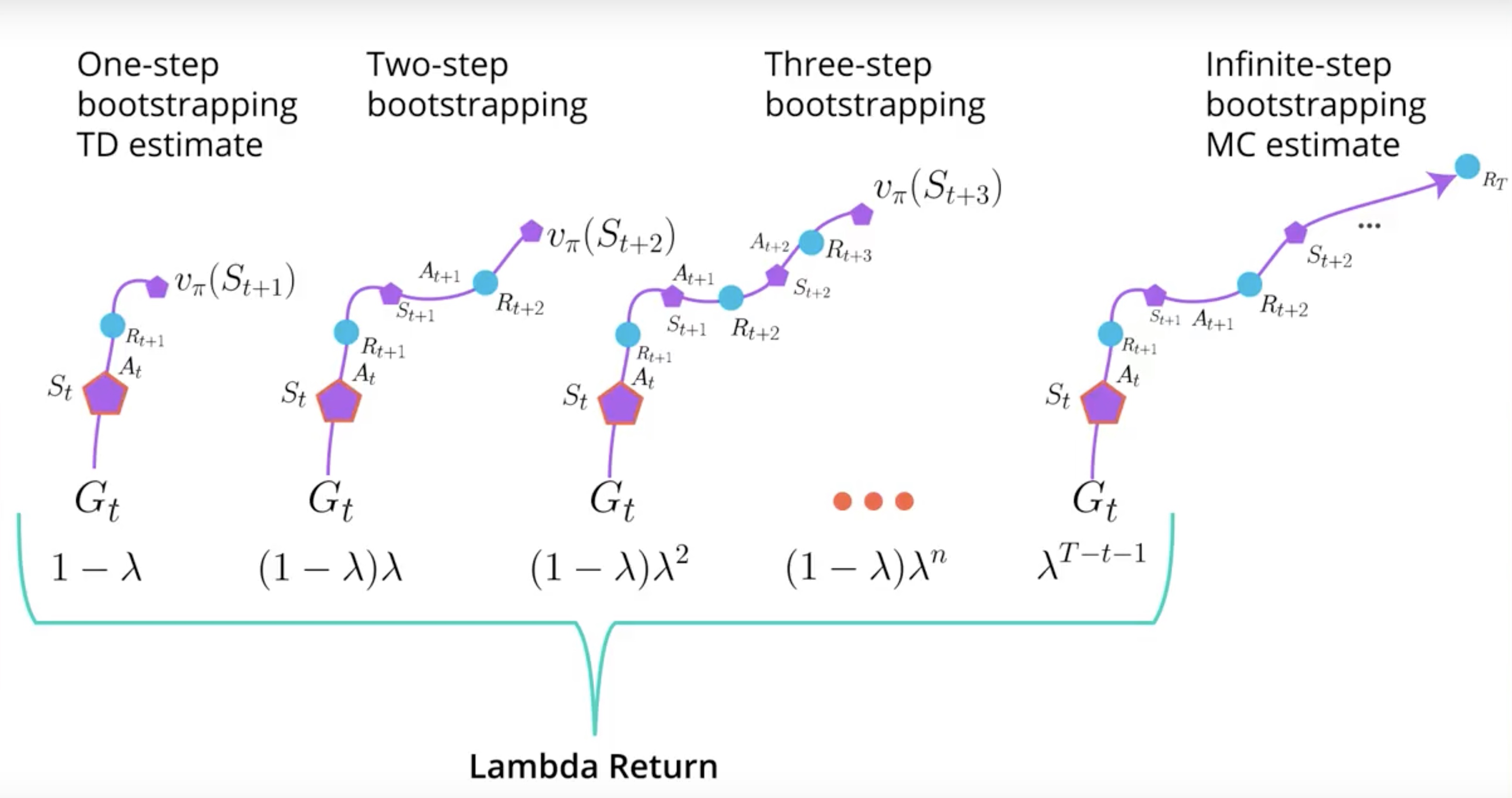
Lamda Return create a mixture of all N-step Bootstrapping estimates at once. Lamda is hyperparameter waiting the combination of each N-step Bootstrapping estimate to the Lamda Return.
from IPython.display import Image
Image(filename='./images/3-4-10-2_gae_lamda_0.5.jpeg')
from IPython.display import Image
Image(filename='./images/3-4-10-3_gae_lamda_0.5_calurate_lamda_return.jpeg')
from IPython.display import Image
Image(filename='./images/3-4-10-4_gae_sum_will_be_the_lamda_return_for_state_s_at_the_time_step_t.jpeg')
from IPython.display import Image
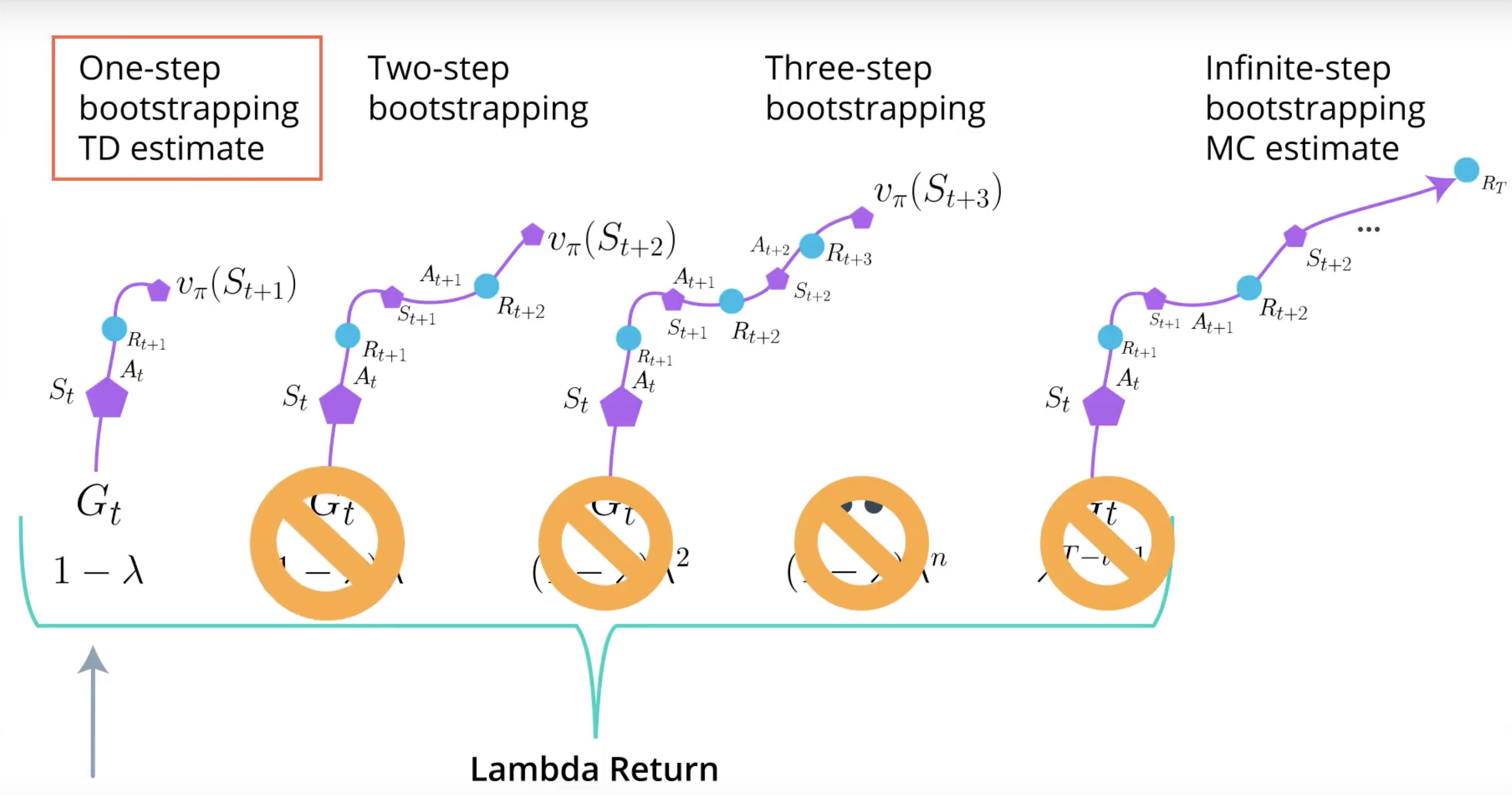
Image(filename='./images/3-4-10-5_gae_lamda_is_one.jpeg')
from IPython.display import Image
Image(filename='./images/3-4-10-6_gae_lamda_is_zero.jpeg')
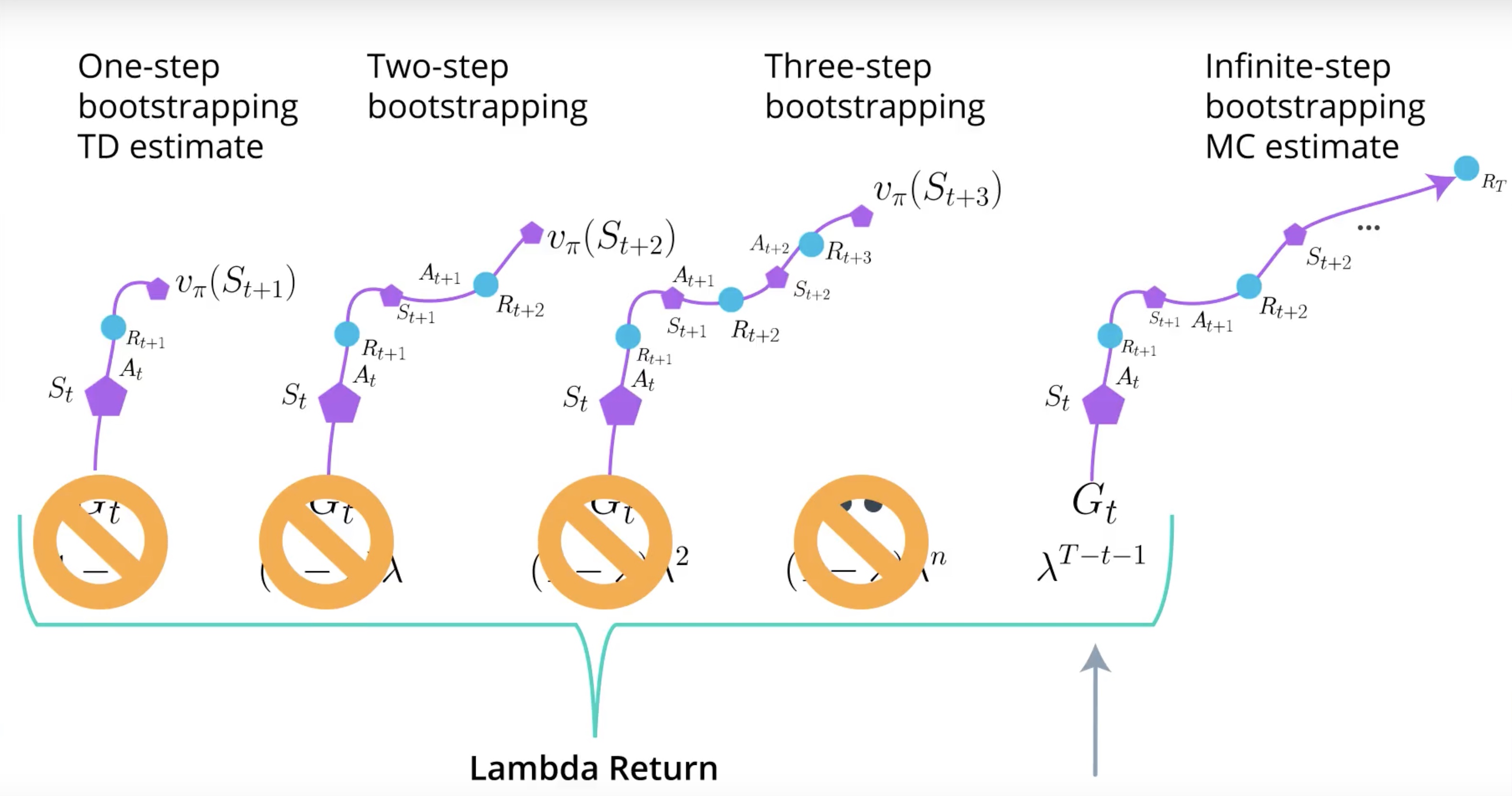
The number between zero and one gives a mixture of all N-step Bootstrapping estimates. It is amazing that a single algorithm do.
GAE is a way to train the Critic with this Lamda Return. You can fit this advantage function in A3C or A2C. but important point is that you can apply GAE to the all kind of Policy-based methods.
Actually The combination of TRPO and GAE train very quickly bacause multiple value functions are spread around on every time step due to Lamda Function.
Link to the GAE paper: https://arxiv.org/abs/1506.02438
3-4-11 : DDPG: Deep Deterministic Policy Gradient, Continuous Action-space
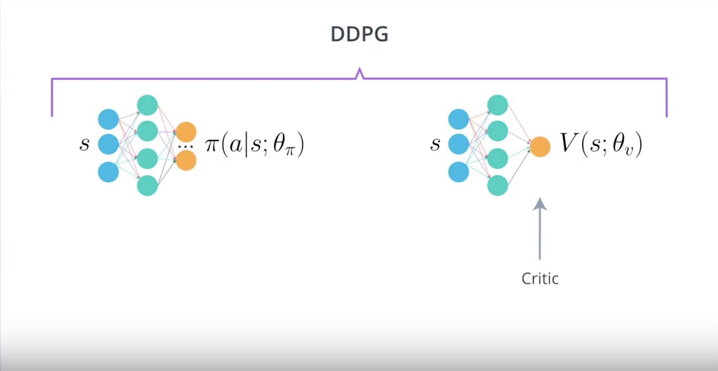
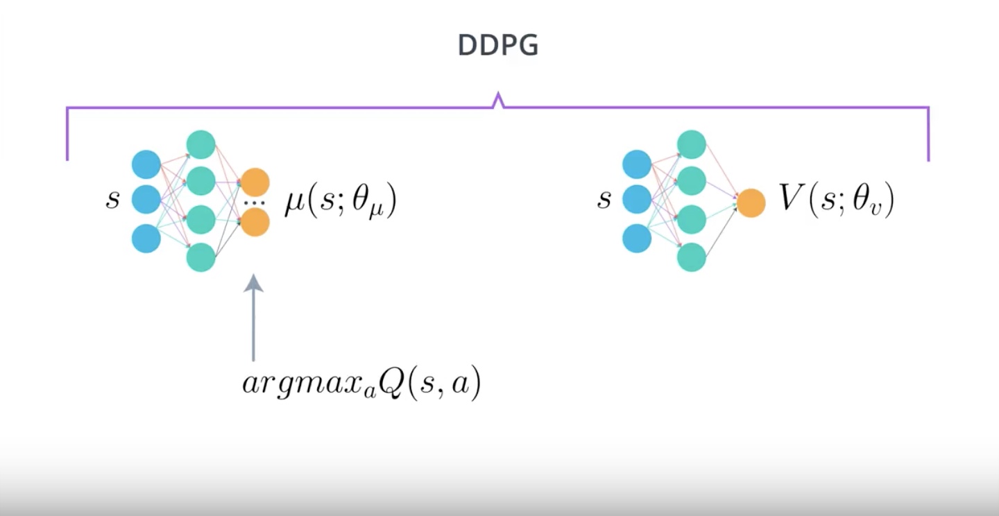
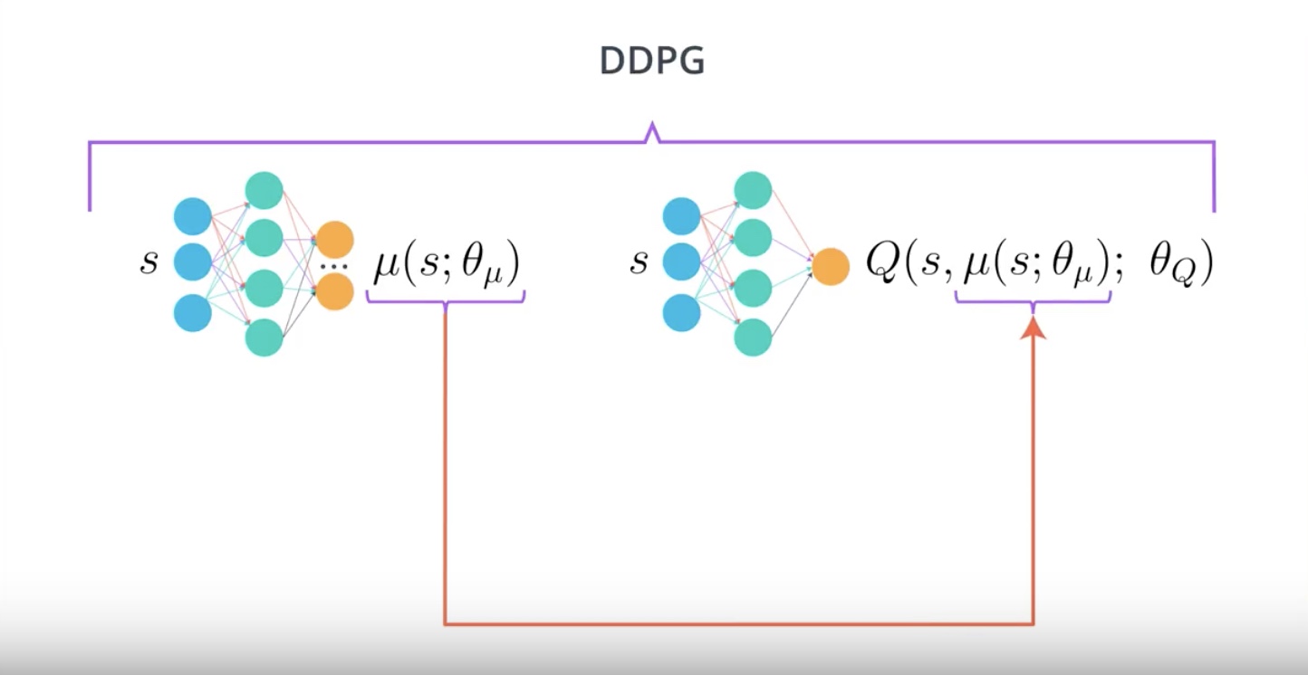
DDPG is a different kind of Actor-Critic Method. It approximate DQN instead of Actor-Critic. Because the Critic in DDPG is used to approximate maximizer over the Q-Value ot the next state. not as a learn as a baseline.
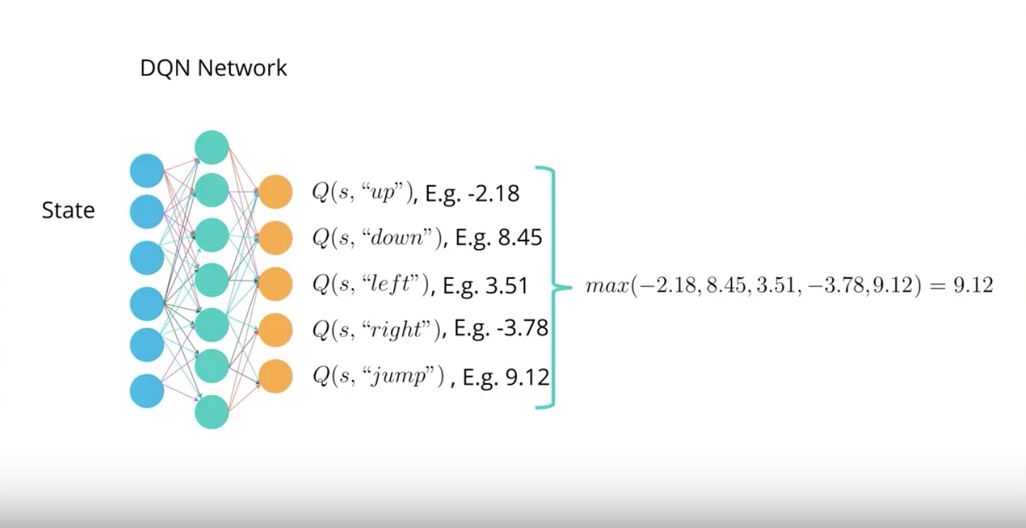
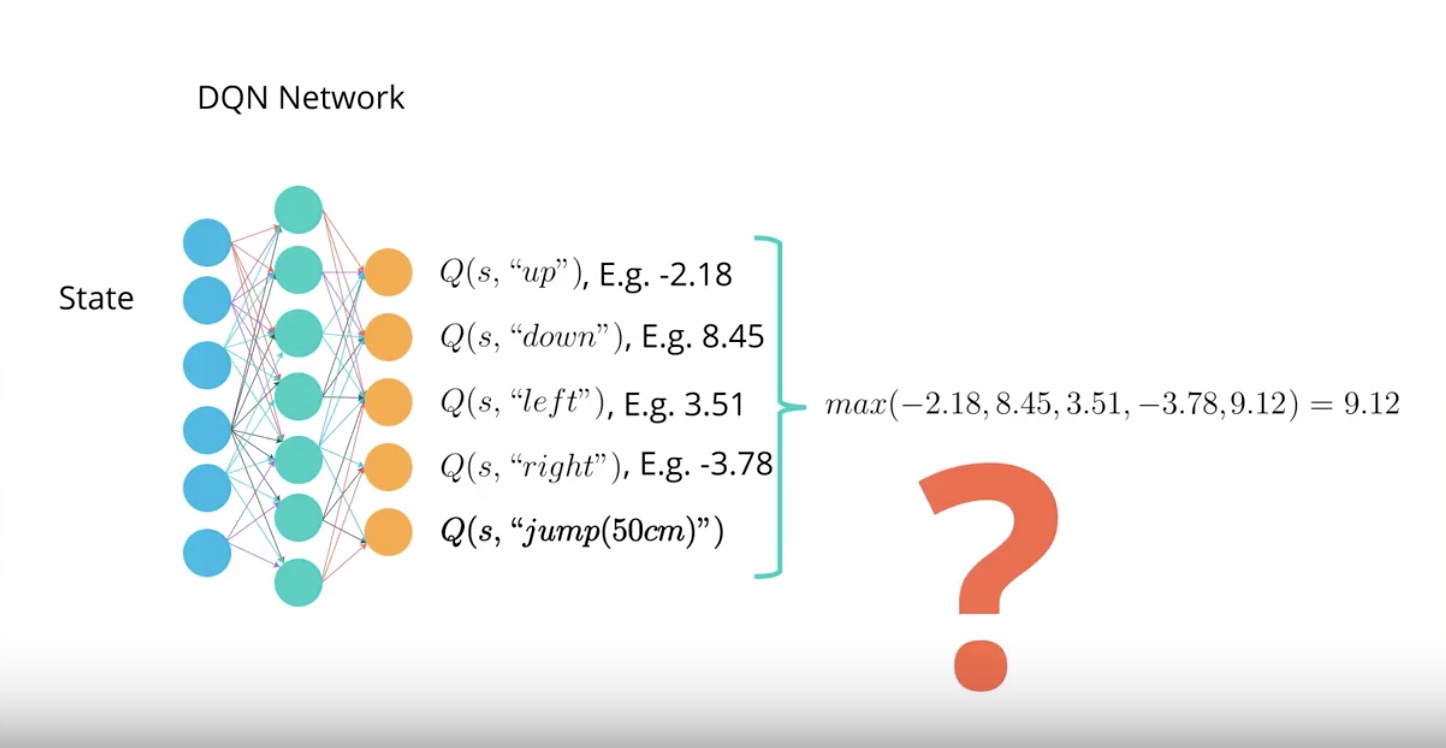
One of the limitation of DQN is that it is not straightfoward in continuous action spaces.
from IPython.display import Image
Image(filename='./images/3-4-11-1_ddpg_descert_action_space_case.jpeg')
from IPython.display import Image
Image(filename='./images/3-4-11-2_ddpg_what_about_continuous_action_space_case.jpeg')
from IPython.display import Image
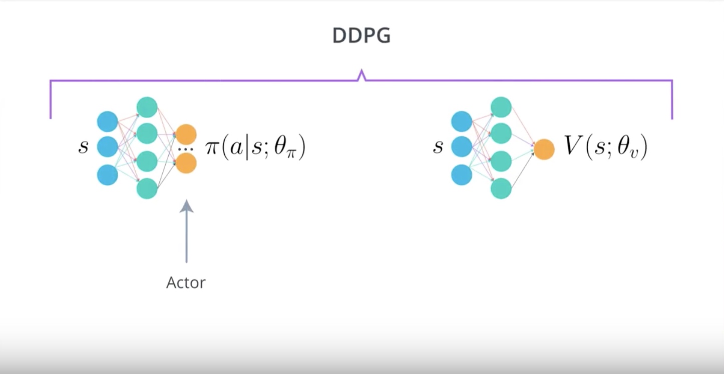
Image(filename='./images/3-4-11-3_ddpg_actor.jpeg')
from IPython.display import Image
Image(filename='./images/3-4-11-4_ddpg_critic.jpeg')
from IPython.display import Image
Image(filename='./images/3-4-11-5_ddpg_actor_changed.jpeg')
from IPython.display import Image
Image(filename='./images/3-4-11-6_ddpg_critic_changed.jpeg')
In the DDPG paper, they introduced this algorithm as an “Actor-Critic” method. Though, some researchers think DDPG is best classified as a DQN method for continuous action spaces (along with NAF). Regardless, DDPG is a very successful method and it’s good for you to gain some intuition.
DDPG paper : https://arxiv.org/abs/1509.02971
NAF paper : https://arxiv.org/abs/1603.00748
3-4-12 : DDPG: Deep Deterministic Policy Gradient, Soft Updates
DDPG uses Replay Buffer.
DDPG uses Soft Update to the target network.
from IPython.display import Image
Image(filename='./images/3-4-11-7_ddpg_dqn_copy_regular_network_weights_to_target_network_every_c_steps.jpeg')
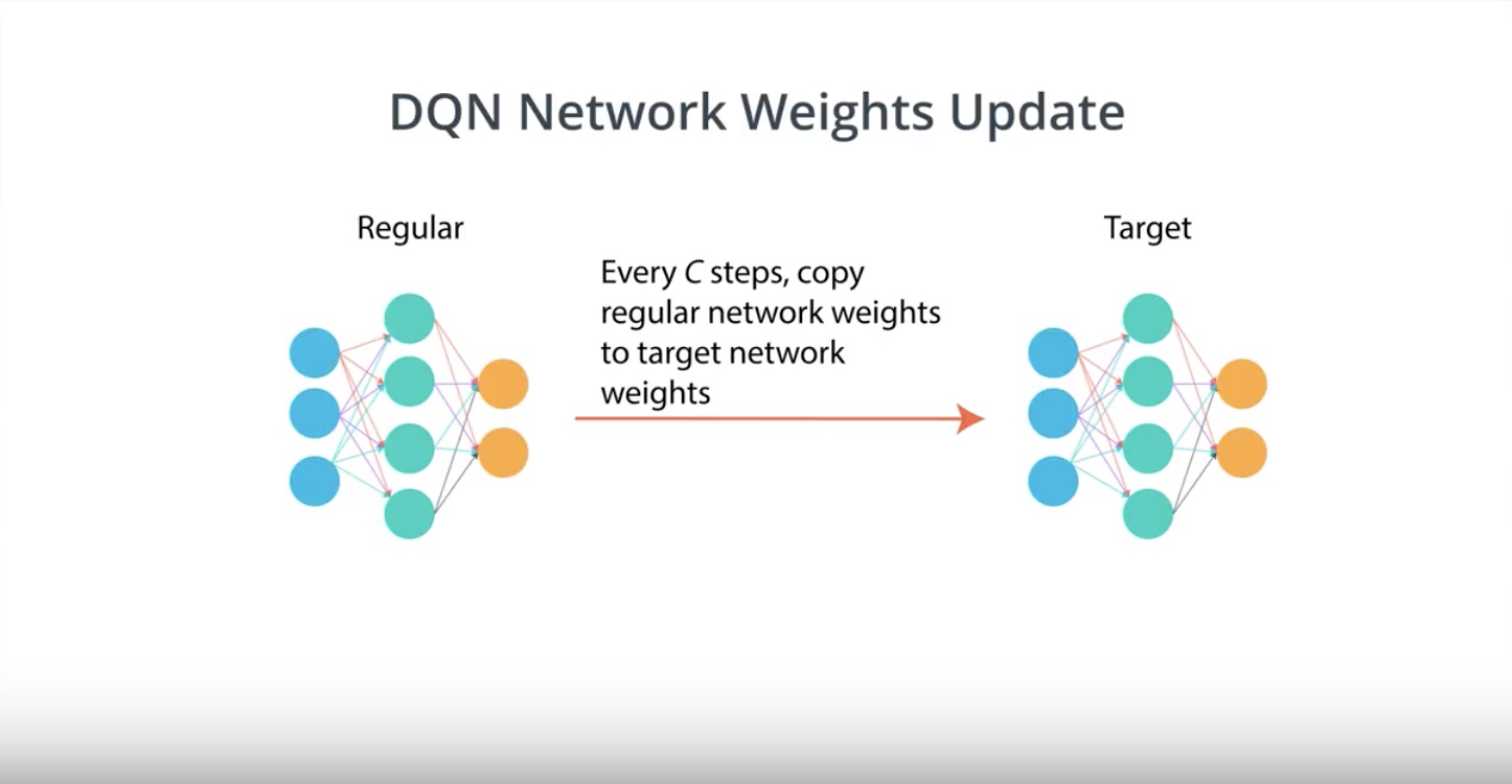
Atari paper says…target network is updated every 10000 time steps…it is so big object.
from IPython.display import Image
Image(filename='./images/3-4-11-8_ddpg_copy_regular_network_weights_to_target_network_by_soft_update_approach.jpeg')
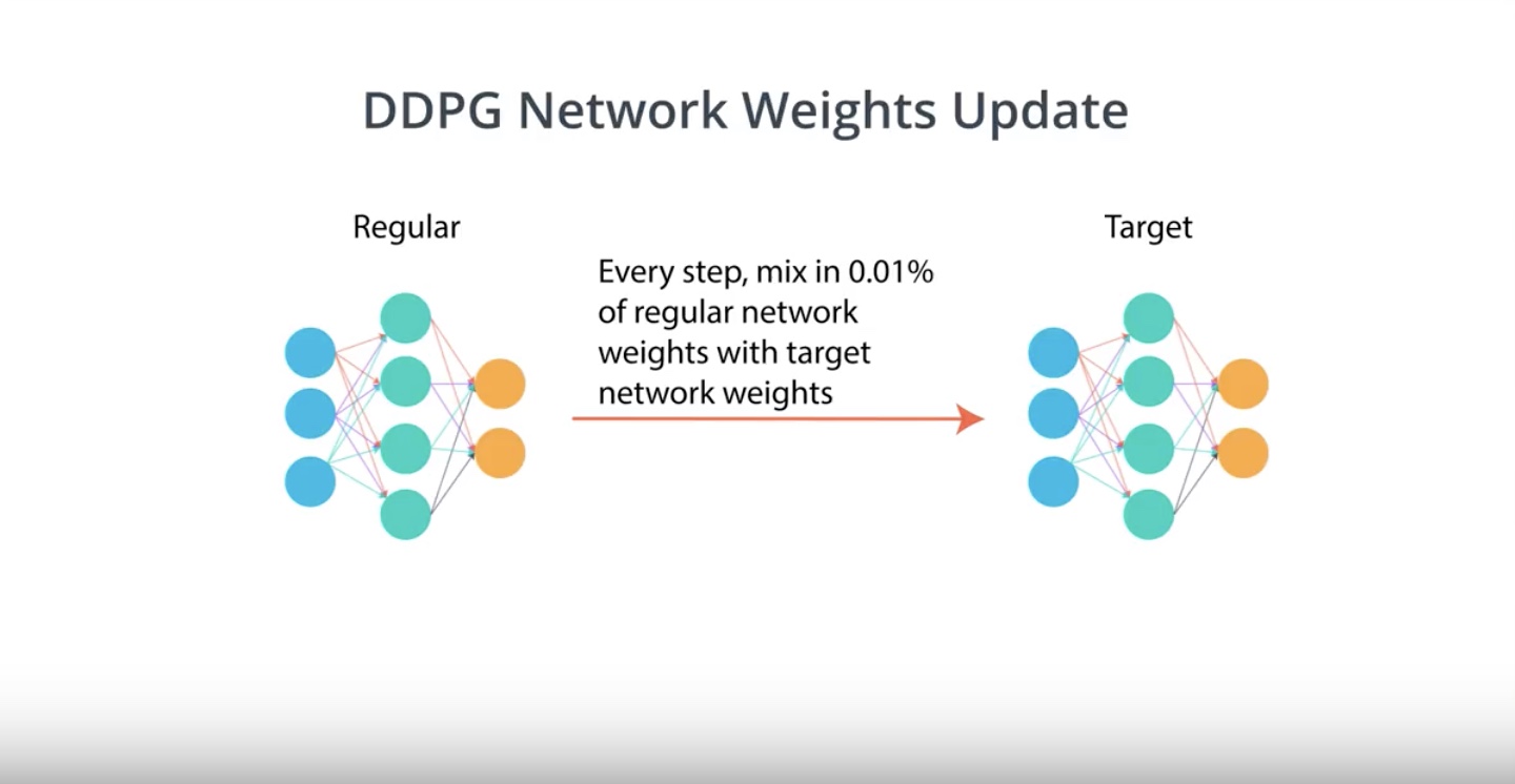
DDPG has 4 Networks.
- Regular Actor network
- Regular Critic network
- Target Actor network
- Target Critic network
Leave a comment