DRL Monte Carlo Mothods

from IPython.display import Image
Image(filename='./images/1-0-0-1_opening.jpg')

Lesson 1-4: Monte Carlo Methods

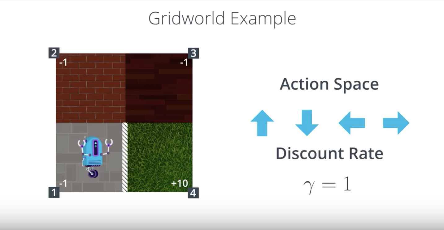
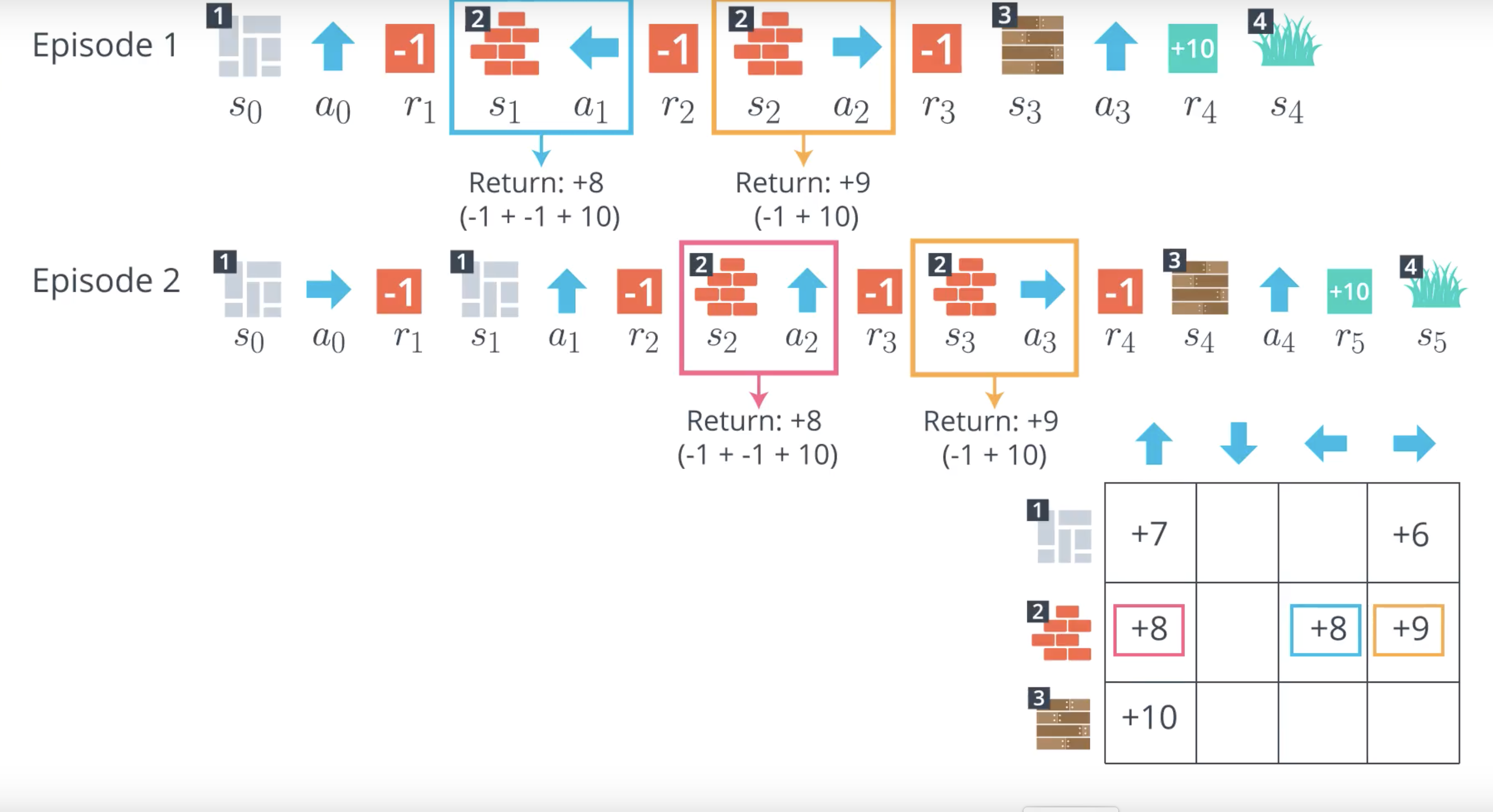
1-4-1 : Gridworld Example

from IPython.display import Image
Image(filename='./images/1-4-1-2_gridworld_example_how_to_choose_action_with_reward.png')

QUESTION 1 OF 5

What is the size of the set S+ of all states (including terminal states)?

1. 2
2. 3
3. 4
4. 5

QUESTION 2 OF 5

What is the size of the set A of all actions?

1. 2
2. 3
3. 4
4. 5

QUESTION 3 OF 5

In the Gridworld Example video, it was mentioned that the discount rate γ=1. With this in mind, which of the following must be true?

1. The agent only cares about the most immediate reward.
2. The reward is not discounted.
3. The agent cares more about future reward than present reward.

QUESTION 4 OF 5

Suppose that at some time step t, the agent is in state 2 and selects action “up”. Which of the following is a possible reward and next state that the agent could receive at time step t+1? (Select all that apply.)

1. reward: -1

   next state: 2

2. reward: 10

   next state: 4

3. reward: -1

   next state: 1

4. reward: -1

   next state: 3

5. reward: 10

   next state: 2

6. reward: -1

   next state: 4

QUESTION 5 OF 5

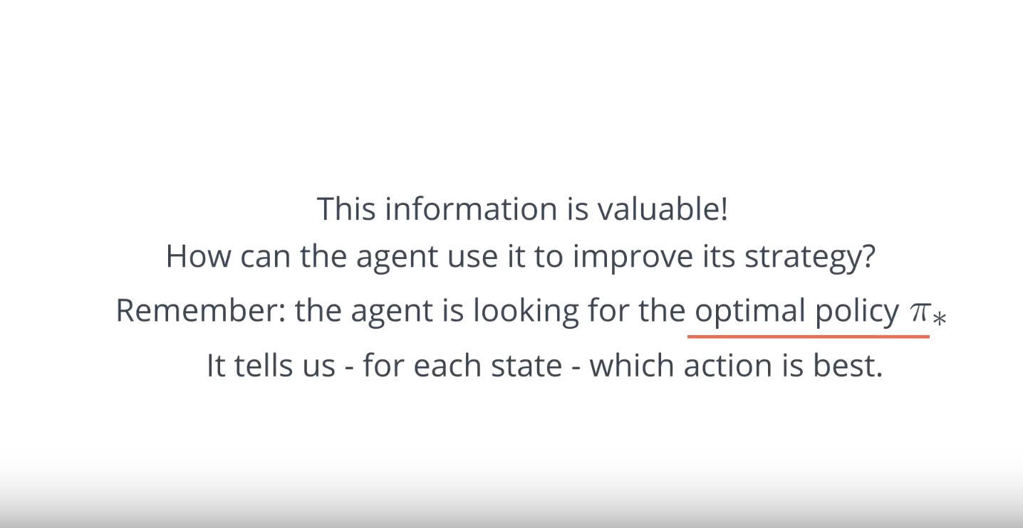
Which of the following choices describes the optimal policy π∗ ?

1. For each state, the agent should randomly select an action, where each action is selected with probability 1/4.
2. The agent should select “up” in state 1, “right” in state 2, and “down” in state 3.
3. The agent should select “down” in state 1, “up” in state 2, and “right” in state 3.
4. The agent should select “right” in state 1, “left” in state 2, and “up” in state 3.

1-4-2 : Monte Carlo Methods

from IPython.display import Image
Image(filename='./images/1-4-2-1_mc_equiprobable_random_policy.png')

from IPython.display import Image
Image(filename='./images/1-4-2-2_mc_equiprobable_random_policy_step1.png')

from IPython.display import Image
Image(filename='./images/1-4-2-3_mc_equiprobable_random_policy_step2.png')

from IPython.display import Image
Image(filename='./images/1-4-2-4_mc_equiprobable_random_policy_step3.png')

from IPython.display import Image
Image(filename='./images/1-4-2-5_mc_equiprobable_random_policy_step4.png')

from IPython.display import Image
Image(filename='./images/1-4-2-6_mc_equiprobable_random_policy_step5.png')

from IPython.display import Image
Image(filename='./images/1-4-2-7_mc_equiprobable_random_policy_step6.png')

from IPython.display import Image
Image(filename='./images/1-4-2-8_mc_equiprobable_random_policy_episode2.png')

from IPython.display import Image
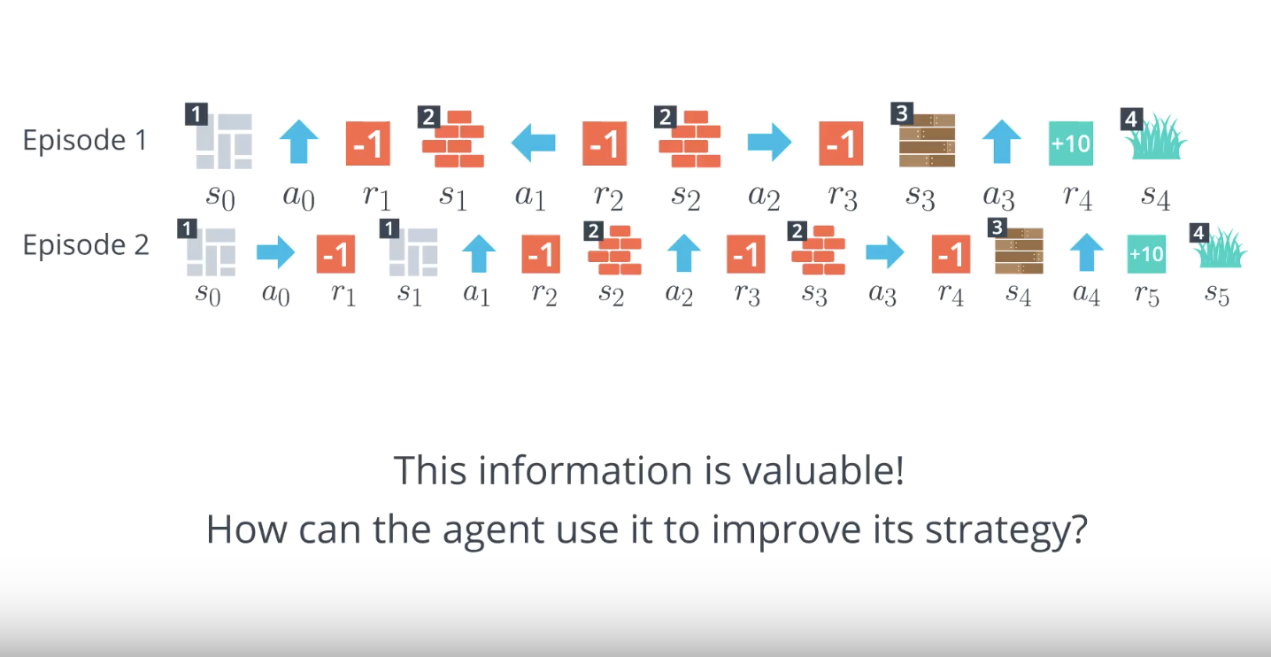
Image(filename='./images/1-4-2-9_mc_equiprobable_random_policy_episodes_are_valuable_imormation.png')

from IPython.display import Image
Image(filename='./images/1-4-2-10_mc_how_can_the_agent_use_episodes_to_improve_its_strategy_?.png')

from IPython.display import Image
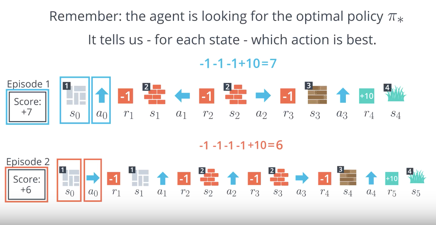
Image(filename='./images/1-4-2-11_mc_each_episode_tells_us_which_action_is_best_for_each_state.png')

from IPython.display import Image
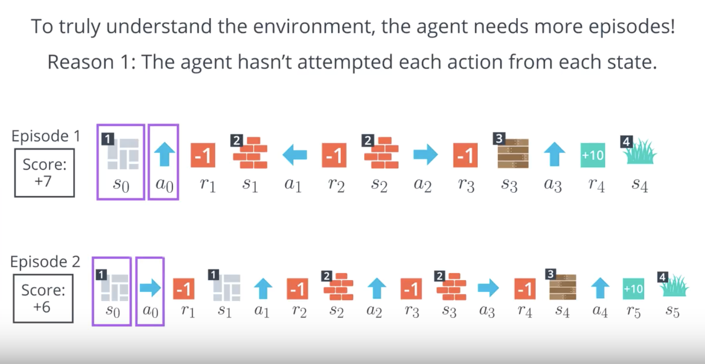
Image(filename='./images/1-4-2-12_mc_the_agent_needs_more_episodes_because_the_agent_hasnot_attempted_each_acton_from_each_state.png')

from IPython.display import Image
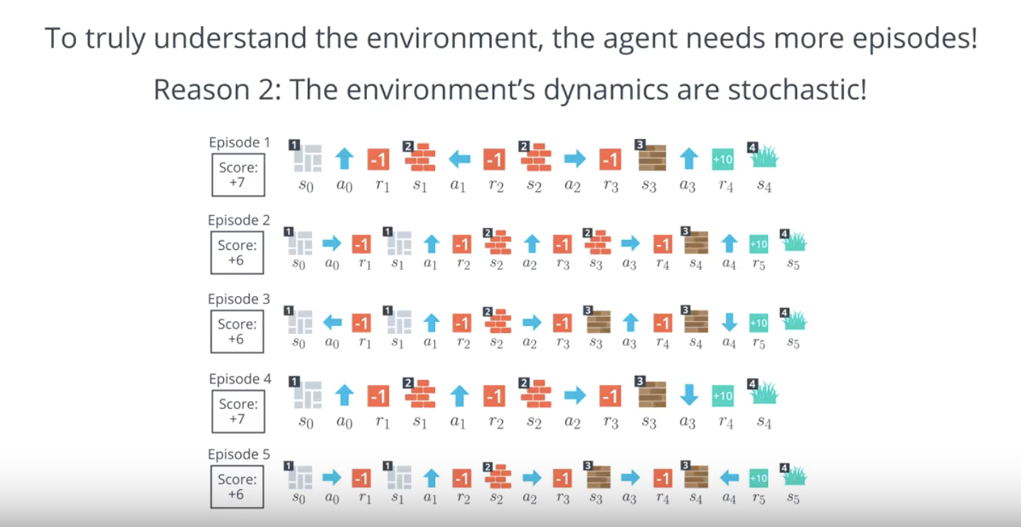
Image(filename='./images/1-4-2-13_mc_reason2_the_environments-dynamics_are_stochastic.png')

from IPython.display import Image
Image(filename='./images/1-4-2-14_mc_reason2_the_environments-dynamics_are_stochastic.png')

from IPython.display import Image
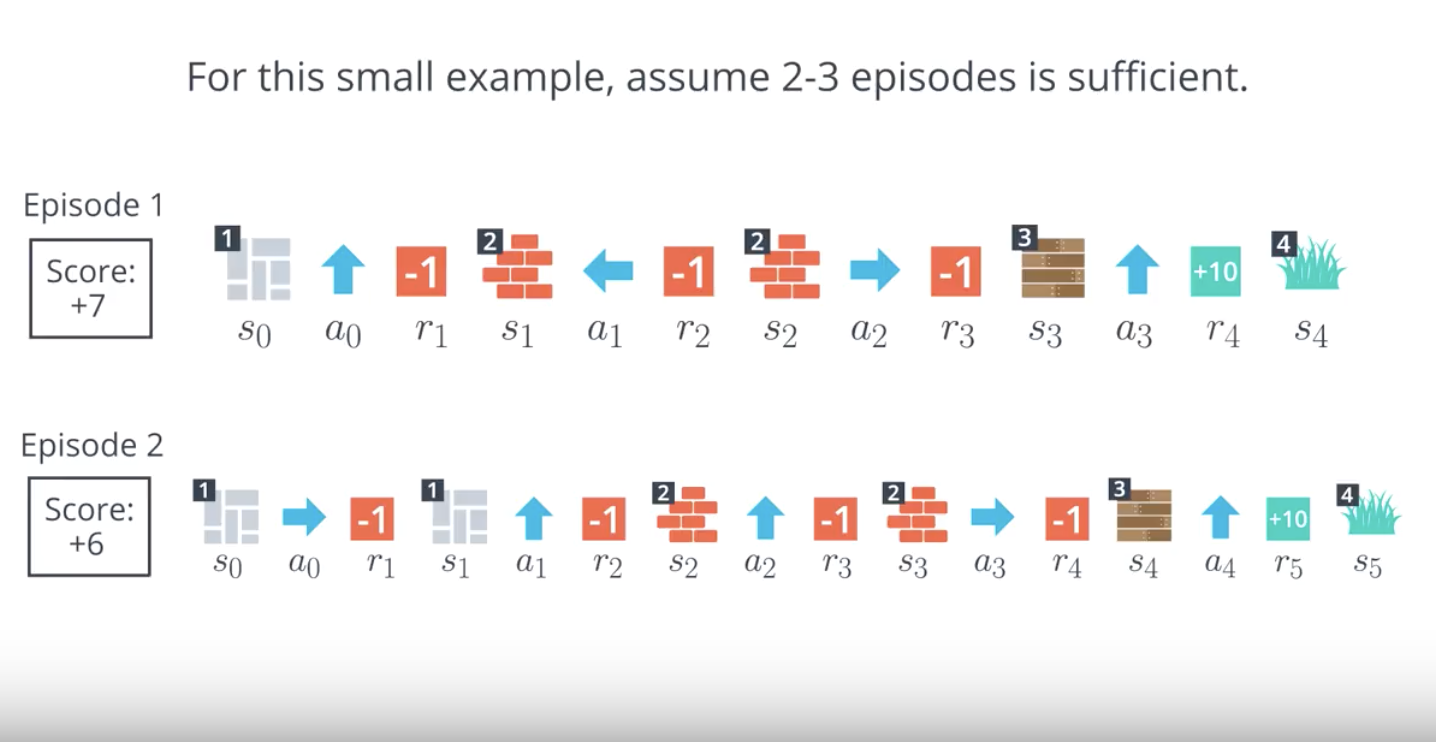
Image(filename='./images/1-4-2-15_mc_for_this_small_example_assume_2_or_3_episodes_is_sufficient.png')

QUIZ QUESTION

Which of the following describes the Monte Carlo approach discussed in the slide obove?

1. After each time step, the agent will select a different action.
2. For the first episode, the agent selects the first action at every time step. For the second episode, it selects a different action, and so on.
3. When the agent has a policy in mind, it follows the policy to collect a lot of episodes. Then, for each state, to figure out which action is best, the agent can look for which action tended to result in the most cumulative reward.
4. When the agent has a policy in mind, it follows the policy to collect a single episode. The agent uses the episode to tell if the policy is good or bad by looking at the cumulative reward that was received by the agent.

1-4-3 : Monte Carlo Prediction

from IPython.display import Image
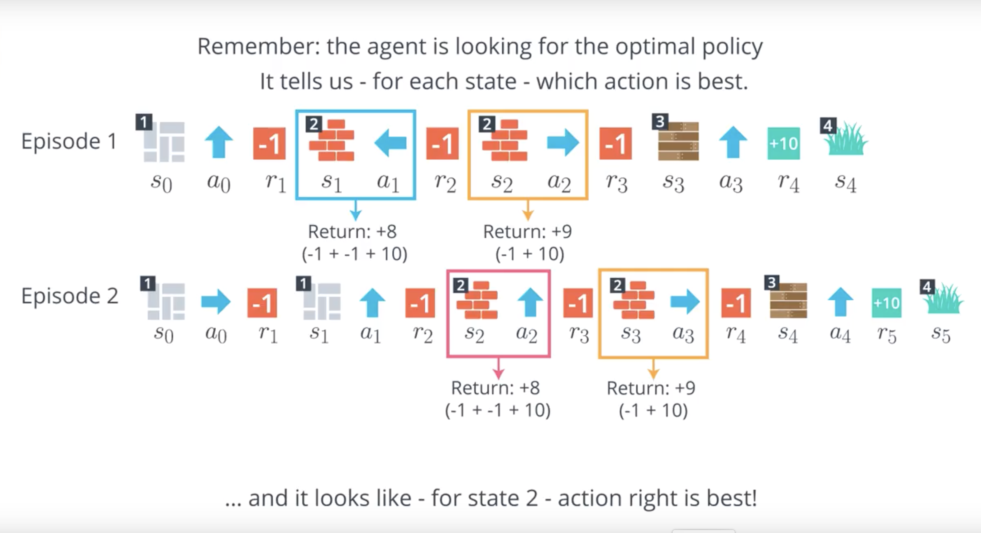
Image(filename='./images/1-4-3-1_mc_prediction_action_right_is_best_for_the_state_2.png')

from IPython.display import Image
Image(filename='./images/1-4-3-2_mc_prediction_we_can_fill_the_table_for_the_remaining_state_action_pairs.png')

from IPython.display import Image
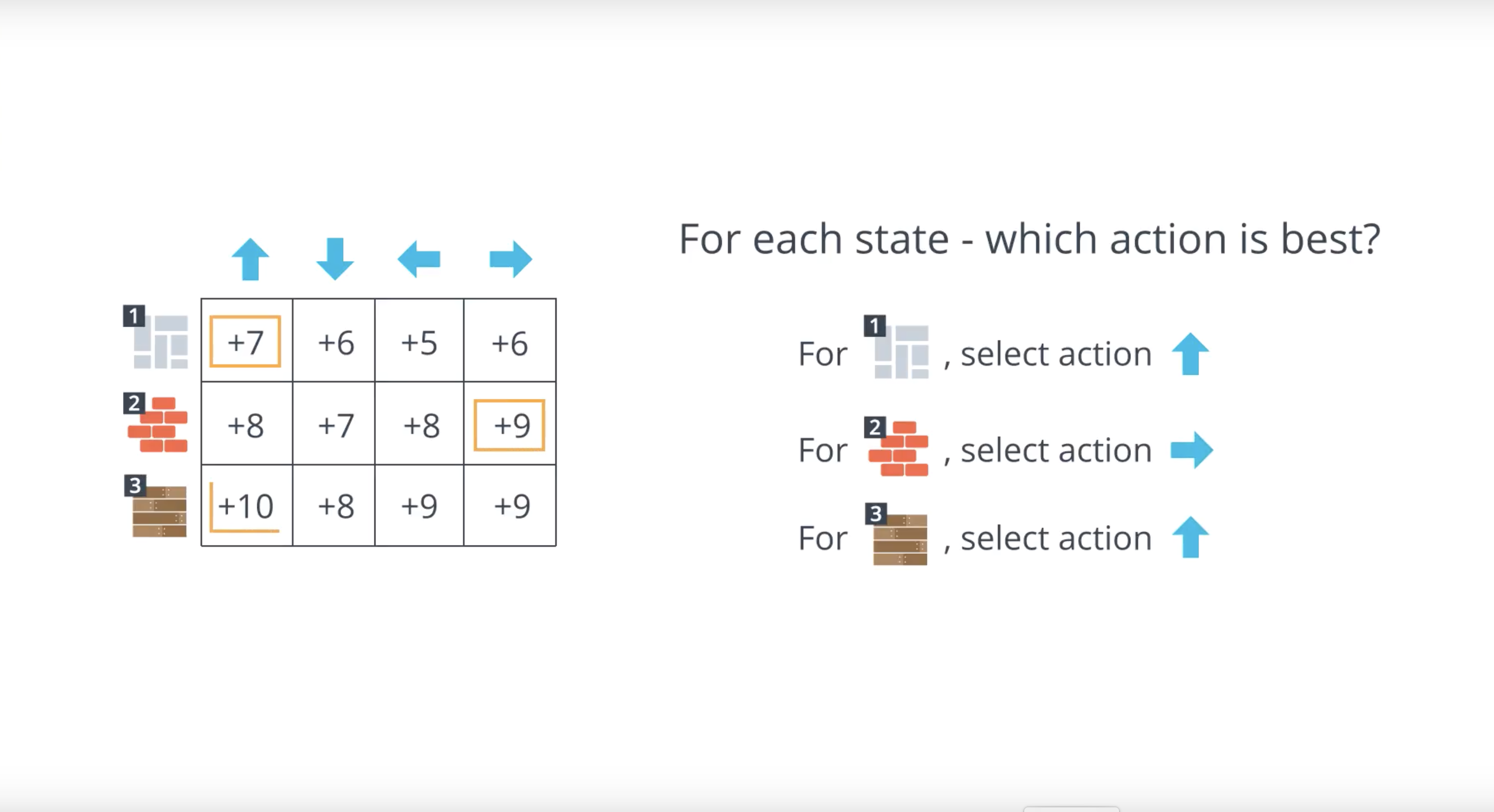
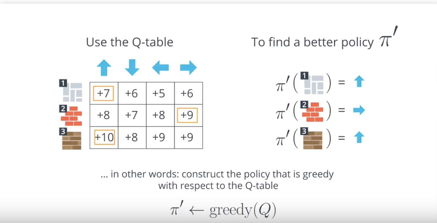
Image(filename='./images/1-4-3-3_mc_prediction_we_can_see_which_action_is_best_for_each_state.png')

from IPython.display import Image
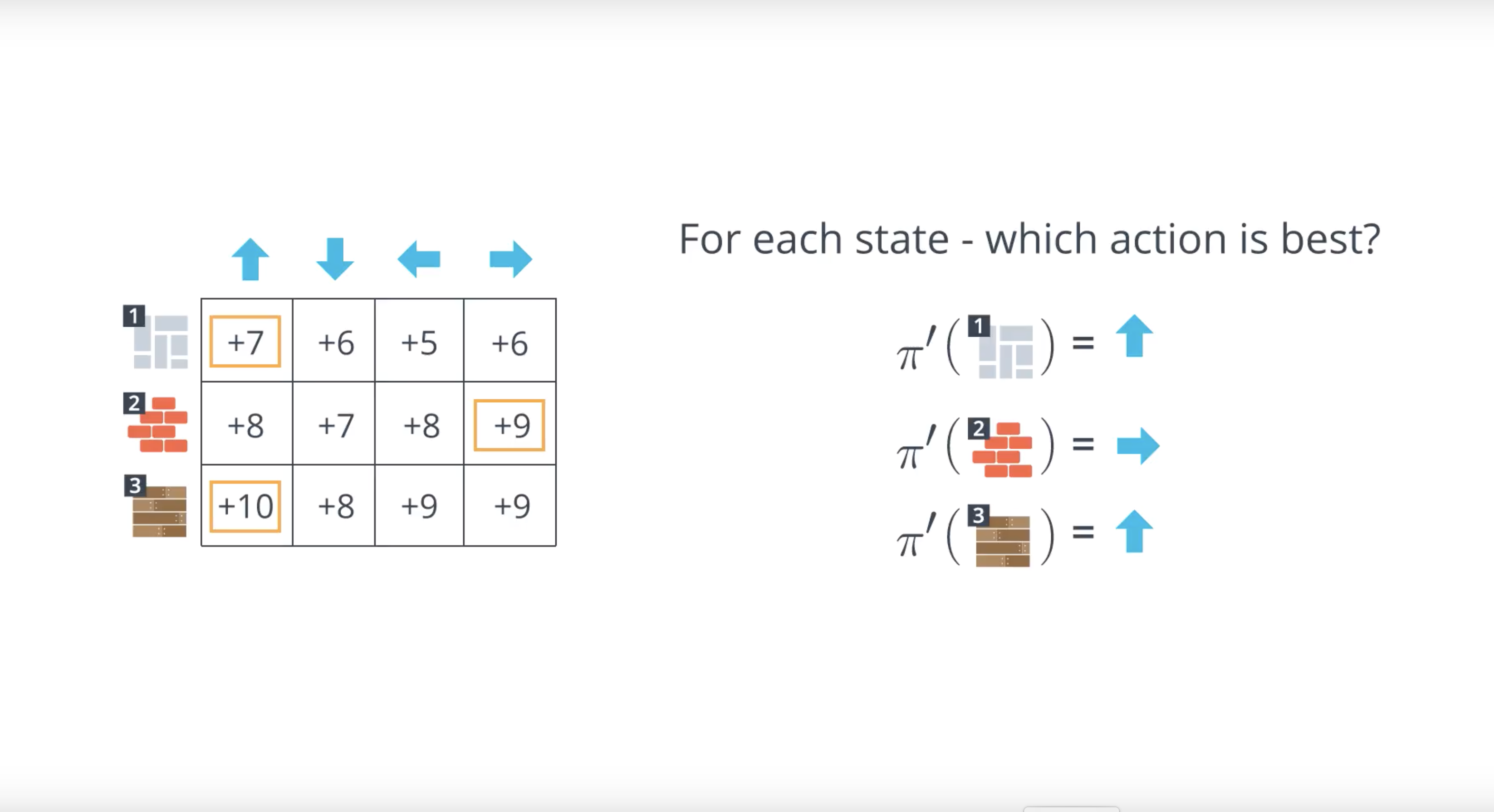
Image(filename='./images/1-4-3-4_mc_prediction_we_denote_this_by_policy_pi_prime_to_distinguish_it_from_previous_policy_pi.png')

from IPython.display import Image
Image(filename='./images/1-4-3-5_mc_prediction_constructing_better_policy_turns_out_tb_be_very_important.png')

Important Note

Above slide, we demonstrated a toy example where the agent collected two episodes, consolidated the information in a table, and then used the table to come up with a better policy. However, as discussed in the previous video, in real-world settings (and even for the toy example depicted here!), the agent will want to collect many more episodes, so that it can better trust the information stored in the table. In this video, we use two episodes only to simplify the example.

from IPython.display import Image
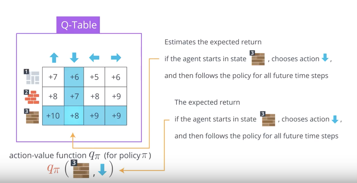
Image(filename='./images/1-4-3-6_mc_prediction_we_use_action_value_function_for_mc_estimation.png')

QUIZ QUESTION

Which of the following is true? (Select all that apply.)

1. If the agent follows a policy for many episodes, we can use the results to directly estimate the action-value function corresponding to the same policy.
2. If the agent knows the equiprobable random policy, we can use it to directly estimate the optimal policy.
3. The Q-table is used to estimate the action-value function.
4. The action-value function is used to estimate the Q-table.

Detailed Explanation for MC Prediction

So far in this lesson, we have discussed how the agent can take a bad policy, like the equiprobable random policy, use it to collect some episodes, and then consolidate the results to arrive at a better policy.

Above slides in the previous concept, you saw that estimating the action-value function with a Q-table is an important intermediate step. We also refer to this as the prediction problem.

Prediction Problem: Given a policy, how might the agent estimate the value function for that policy?

We’ve been specifically interested in the action-value function, but the prediction problem also refers to approaches that can be used to estimate the state-value function. We refer to Monte Carlo (MC) approaches to the prediction problem as MC prediction methods.

Pseudocode

As you have learned above slides, in the algorithm for MC prediction, we begin by collecting many episodes with the policy. Then, we note that each entry in the Q-table corresponds to a particular state and action. To populate an entry, we use the return that followed when the agent was in that state, and chose the action. In the event that the agent has selected the same action many times from the same state, we need only average the returns.

Before we dig into the pseudocode, we note that there are two different versions of MC prediction, depending on how you decide to treat the special case where - in a single episode - the same action is selected from the same state many times.

from IPython.display import Image
Image(filename='./images/1-4-3-7_mc_prediction_there_are_two_options.png')

from IPython.display import Image
Image(filename='./images/1-4-3-8_mc_prediction_every-visit-mc_and_first-visit-mc.png')

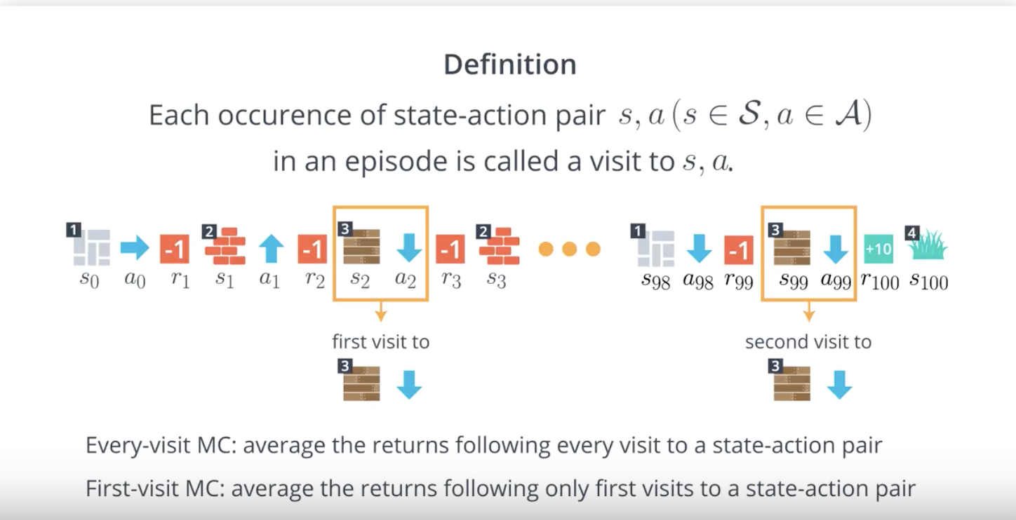
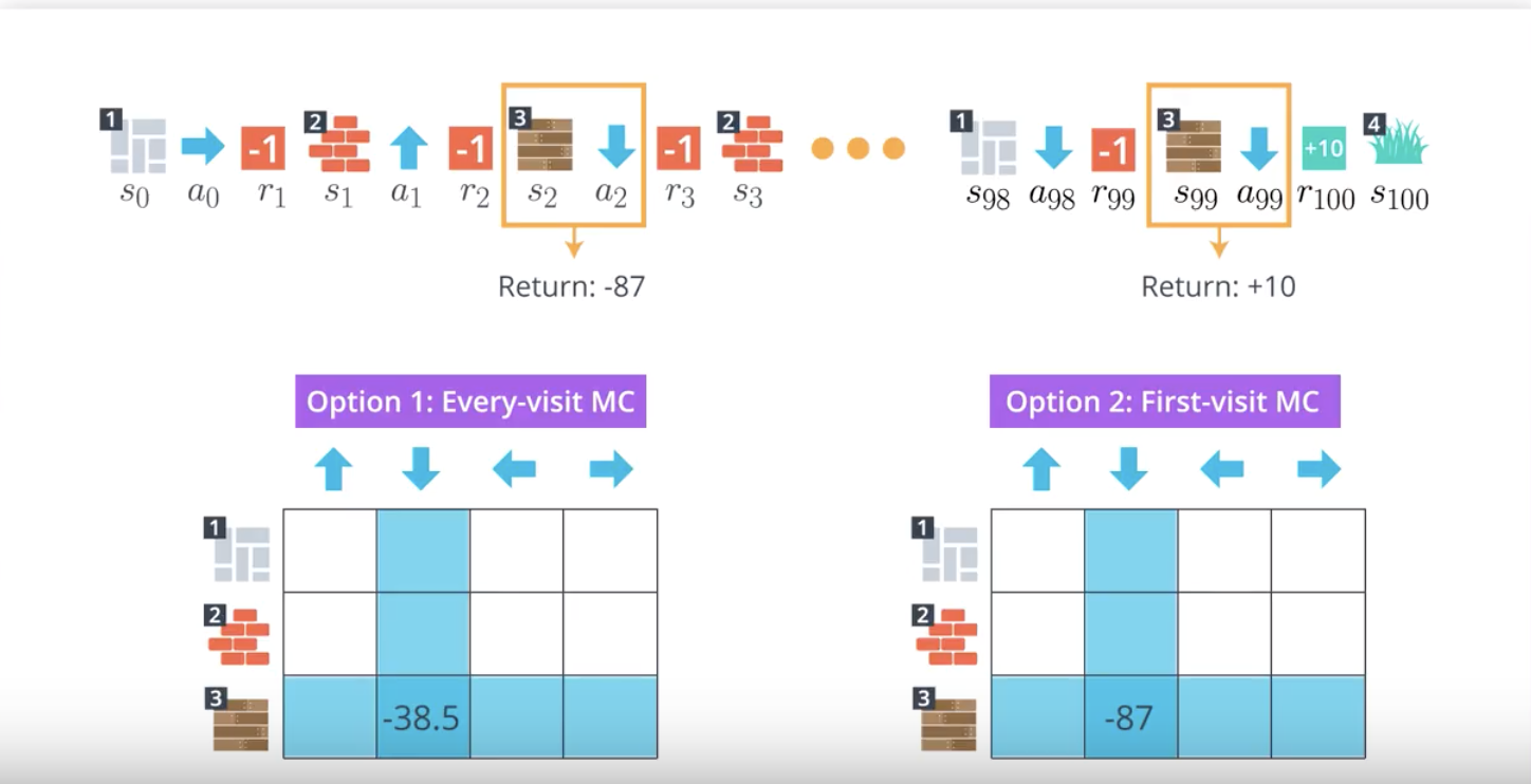
As discussed above slides, we define every occurrence of a state in an episode as a visit to that state-action pair. And, in the event that a state-action pair is visited more than once in an episode, we have two options.

Option 1: Every-visit MC Prediction

Average the returns following all visits to each state-action pair, in all episodes.

Option 2: First-visit MC Prediction

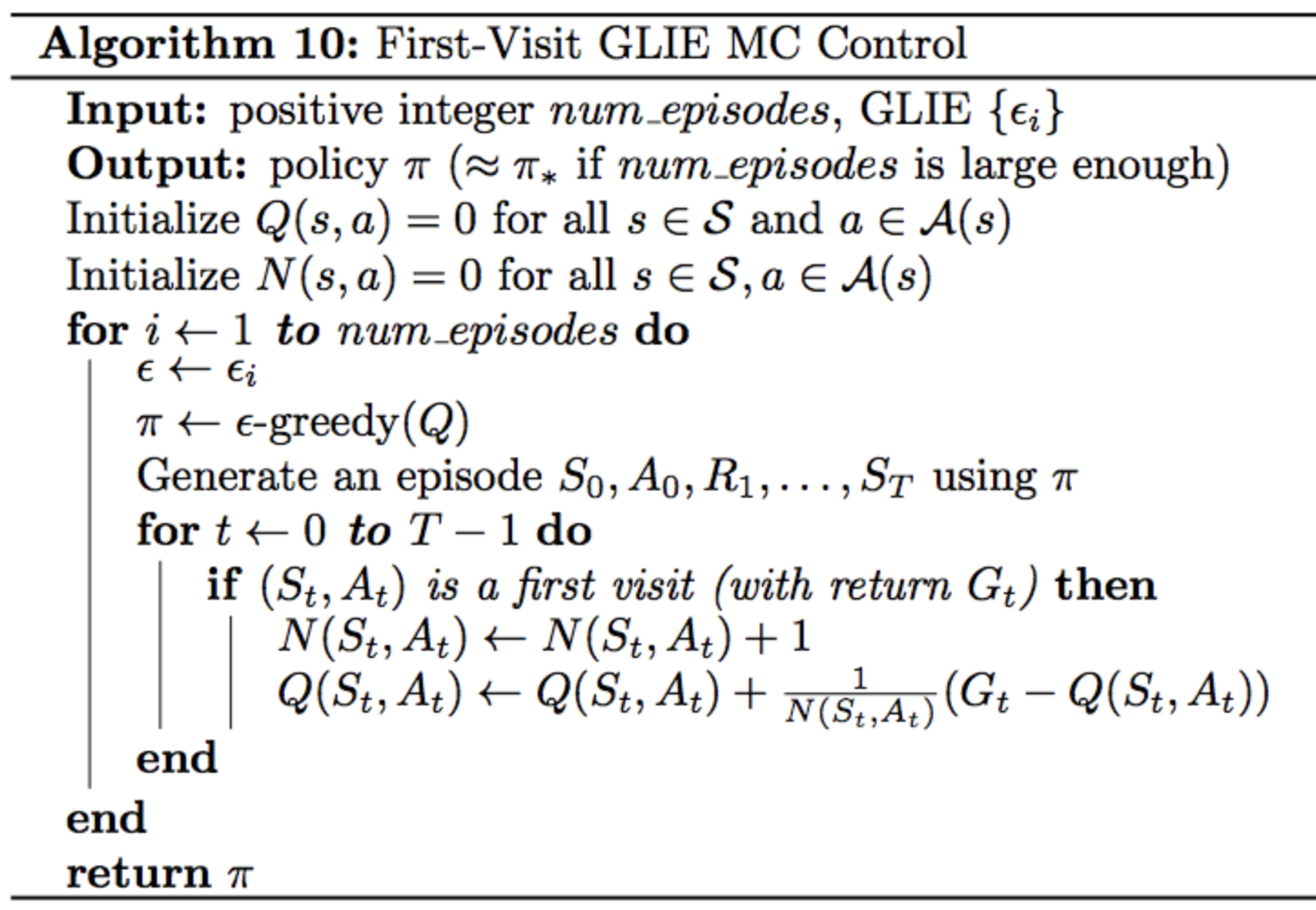
For each episode, we only consider the first visit to the state-action pair. The pseudocode for this option can be found below.

from IPython.display import Image
Image(filename='./images/1-4-3-9_mc_prediction_first-visit-mc_peusocode.png')

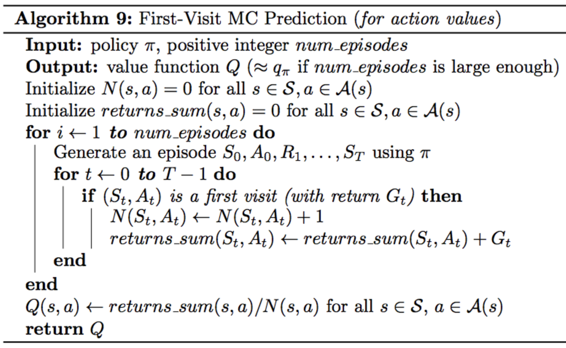
Don’t let this pseudocode scare you! The main idea is quite simple. There are three relevant tables:

• Q - Q-table, with a row for each state and a column for each action. The entry corresponding to state s and action a is denoted Q(s,a).
• N - table that keeps track of the number of first visits we have made to each state-action pair.
• returns_sum - table that keeps track of the sum of the rewards obtained after first visits to each state-action pair.

In the algorithm, the number of episodes the agent collects is equal to num_episodes. After each episode, N and returns_sum are updated to store the information contained in the episode. Then, after all of the episodes have been collected and the values in N and returns_sum have been finalized, we quickly obtain the final estimate for Q.

Soon, you’ll have the chance to implement this algorithm yourself!

You will apply your code to OpenAI Gym’s BlackJack environment. Note that in the game of BlackJack, first-visit and every-visit MC return identical results!

First-visit or Every-visit?

Both the first-visit and every-visit method are guaranteed to converge to the true action-value function, as the number of visits to each state-action pair approaches infinity. (So, in other words, as long as the agent gets enough experience with each state-action pair, the value function estimate will be pretty close to the true value.) In the case of first-visit MC, convergence follows from the Law of Large Numbers, and the details are covered in section 5.1 of the Sutton’s textbook.

If you are interested in learning more about the difference between first-visit and every-visit MC methods, you are encouraged to read Section 3 of this paper. The results are summarized in Section 3.6. The authors show:

Every-visit MC is biased, whereas first-visit MC is unbiased (see Theorems 6 and 7). Initially, every-visit MC has lower mean squared error (MSE), but as more episodes are collected, first-visit MC attains better MSE (see Corollary 9a and 10a, and Figure 4).

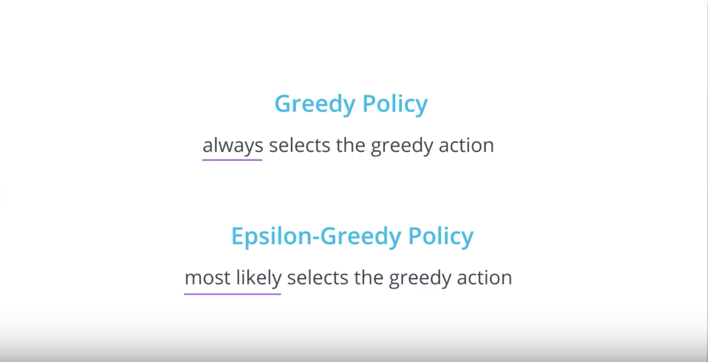
1-4-4 : Greedy Policies

from IPython.display import Image
Image(filename='./images/1-4-4-1_greed_policy.png')

from IPython.display import Image
Image(filename='./images/1-4-4-2_greed_policy.png')

from IPython.display import Image
Image(filename='./images/1-4-4-3_greed_policy.png')

Quiz

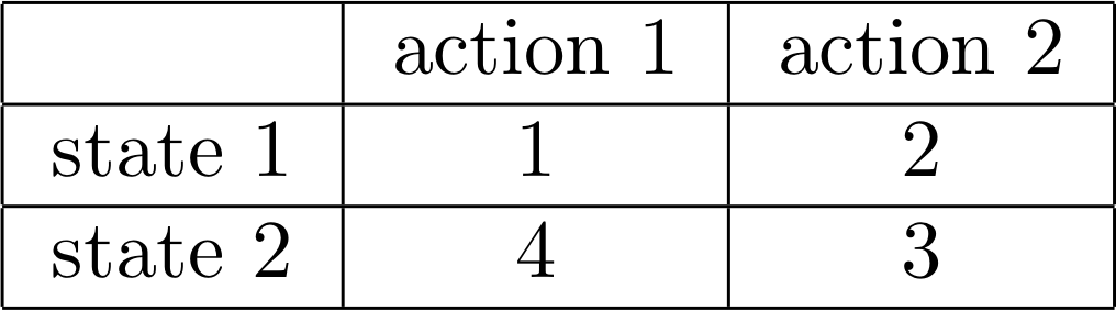
An example of a Q-table is provided below.

from IPython.display import Image
Image(filename='./images/1-4-4-4_greed_policy_quiz_q_table.png')

QUIZ QUESTION

Which of the following describes the policy that is greedy with respect to the Q-table?

1. In state 1, select action 1. In state 2, select action 1.
2. In state 1, select action 1. In state 2, select action 2.
3. In state 1, select action 2. In state 2, select action 1.
4. In state 1, select action 2. In state 2, select action 2.

1-4-5 : Epsilon-Greedy Policies

from IPython.display import Image
Image(filename='./images/1-4-5-1_e_greed_policy.png')

from IPython.display import Image
Image(filename='./images/1-4-5-2_e_greed_policy.png')

from IPython.display import Image
Image(filename='./images/1-4-5-3_e_greed_policy.png')

Note

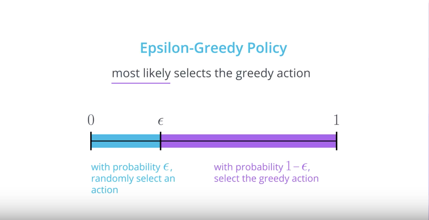
In the above slides, you learned about ϵ-greedy policies.

You can think of the agent who follows an ϵ-greedy policy as always having a (potentially unfair) coin at its disposal, with probability ϵ of landing heads. After observing a state, the agent flips the coin.

If the coin lands tails (so, with probability 1−ϵ), the agent selects the greedy action. If the coin lands heads (so, with probability ϵ), the agent selects an action uniformly at random from the set of available (non-greedy AND greedy) actions. In order to construct a policy π that is ϵ-greedy with respect to the current action-value function estimate Q, we will set

from IPython.display import Image
Image(filename='./images/1-4-5-4_e_greed_policy.png')

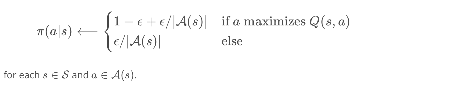
Mathematically, A(s) is the set of all possible actions at state s (which may be ‘up’, ‘down’,’right’, ‘left’ for example), and ∣A(s)∣ the number of possible actions (including the optimal one!). The reason why we include an extra term ϵ/∣A(s)∣ for the optimal action is because the sum of all the probabilities needs to be 1. If we sum over the probabilities of performing non-optimal actions, we will get (∣A(s)∣−1)×ϵ/∣A(s)∣, and adding this to 1−ϵ+ϵ/∣A(s)∣ gives one.

Note that ϵ must always be a value between 0 and 1, inclusive (that is, ϵ∈[0,1]).

QUESTION 1 OF 4

Which of the values for epsilon yields an epsilon-greedy policy that is guaranteed to always select the greedy action? Select all that apply.

• (1) epsilon = 0
• (2) epsilon = 0.3
• (3) epsilon = 0.5
• (4) epsilon = 1
• (5) This is a trick question! The true answer is that none of the values for epsilon satisfy this requirement.

QUESTION 2 OF 4

Which of the values for epsilon yields an epsilon-greedy policy that is guaranteed to always select a non-greedy action? Select all that apply.

• (1) epsilon = 0
• (2) epsilon = 0.3
• (3) epsilon = 0.5
• (4) epsilon = 1
• (5) This is a trick question! The true answer is that none of the values for epsilon satisfy this requirement.

QUESTION 3 OF 4

Which of the values for epsilon yields an epsilon-greedy policy that is equivalent to the equiprobable random policy (where, from each state, each action is equally likely to be selected)?

• (1) epsilon = 0
• (2) epsilon = 0.3
• (3) epsilon = 0.5
• (4) epsilon = 1
• (5) This is a trick question! The true answer is that none of the values for epsilon satisfy this requirement.

QUESTION 4 OF 4

Which of the values for epsilon yields an epsilon-greedy policy where the agent has the possibility of selecting a greedy action, but might select a non-greedy action instead? In other words, how might you guarantee that the agent selects each of the available (greedy and non-greedy) actions with nonzero probability?

• (1) epsilon = 0
• (1) epsilon = 0
• (2) epsilon = 0.3
• (3) epsilon = 0.5
• (4) epsilon = 1
• (5) This is a trick question! The true answer is that none of the values for epsilon satisfy this requirement.

1-4-6 : Monte Carlo Control

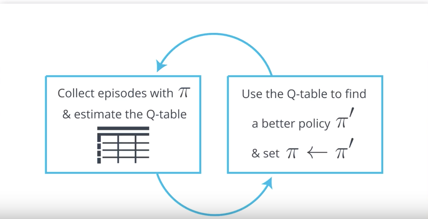
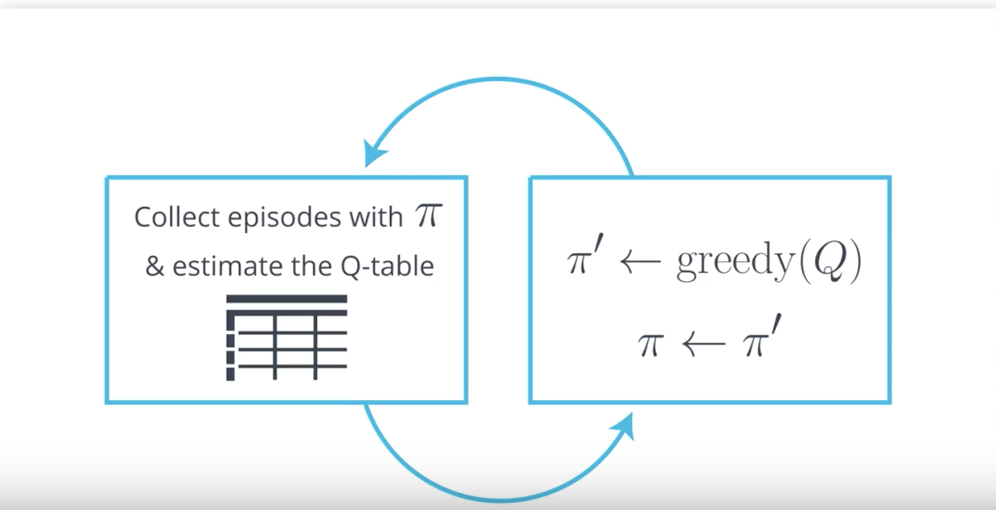
So far, you have learned how the agent can take a policy π, use it to interact with the environment for many episodes, and then use the results to estimate the action-value function qπ with a Q-table.

Then, once the Q-table closely approximates the action-value function qπ, the agent can construct the policy π′ that is ϵ-greedy with respect to the Q-table, which will yield a policy that is better than the original policy π.

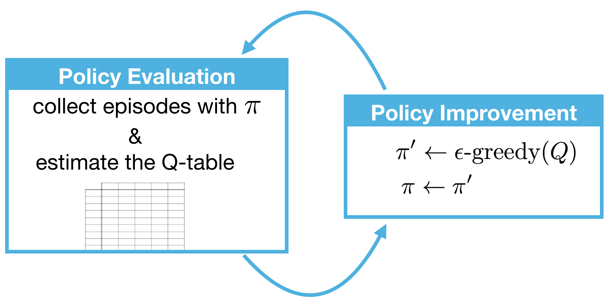
Furthermore, if the agent alternates between these two steps, with:

• Step 1: using the policy π to construct the Q-table, and
• Step 2: improving the policy by changing it to be ϵ-greedy with respect to the Q-table (π′←ϵ-greedy(Q), π←π′),

we will eventually obtain the optimal policy π∗.

Since this algorithm is a solution for the control problem (defined below), we call it a Monte Carlo control method.

Control Problem: Estimate the optimal policy.

It is common to refer to Step 1 as policy evaluation, since it is used to determine the action-value function of the policy. Likewise, since Step 2 is used to improve the policy, we also refer to it as a policy improvement step.

So, using this new terminology, we can summarize what we’ve learned to say that our Monte Carlo control method alternates between policy evaluation and policy improvement steps to recover the optimal policy π∗.

from IPython.display import Image
Image(filename='./images/1-4-6-1_mc_control.png')

1-4-7 : Exploration vs. Exploitation

Solving Environments in OpenAI Gym

In many cases, we would like our reinforcement learning (RL) agents to learn to maximize reward as quickly as possible. This can be seen in many OpenAI Gym environments.

For instance, the FrozenLake-v0 environment is considered solved once the agent attains an average reward of 0.78 over 100 consecutive trials.

from IPython.display import Image
Image(filename='./images/1-4-7-1_exploration_vs_exploitation.png')

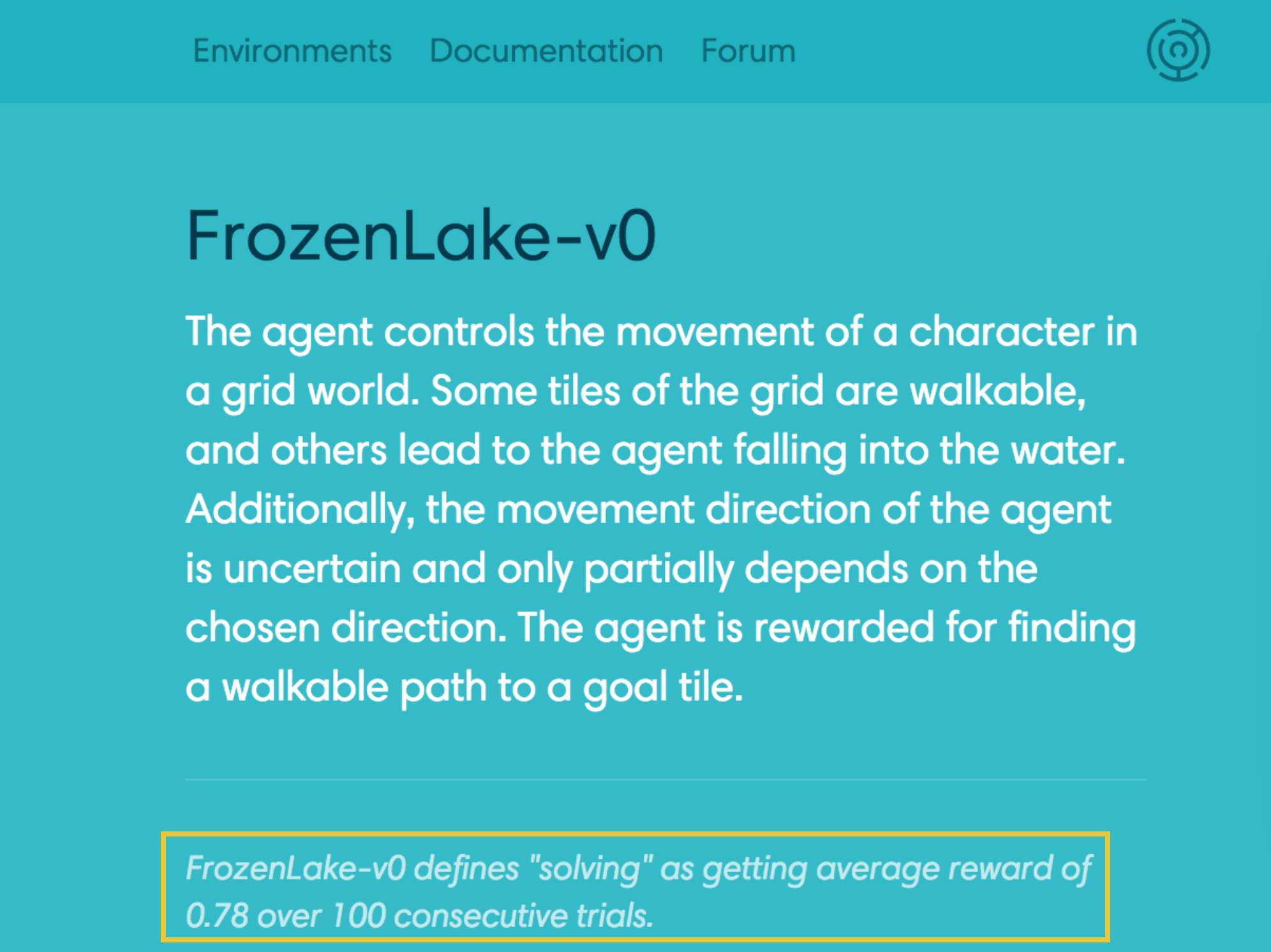
Algorithmic solutions to the FrozenLake-v0 environment are ranked according to the number of episodes needed to find the solution.

from IPython.display import Image
Image(filename='./images/1-4-7-2_exploration_vs_exploitation.png')

Solutions to Taxi-v1, Cartpole-v1, and MountainCar-v0 (along with many others) are also ranked according to the number of episodes before the solution is found. Towards this objective, it makes sense to design an algorithm that learns the optimal policy π∗ as quickly as possible.

Exploration-Exploitation Dilemma

Recall that the environment’s dynamics are initially unknown to the agent. Towards maximizing return, the agent must learn about the environment through interaction.

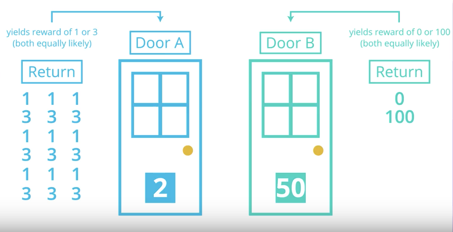
At every time step, when the agent selects an action, it bases its decision on past experience with the environment. And, towards minimizing the number of episodes needed to solve environments in OpenAI Gym, our first instinct could be to devise a strategy where the agent always selects the action that it believes (based on its past experience) will maximize return. With this in mind, the agent could follow the policy that is greedy with respect to the action-value function estimate. We examined this approach in a previous slides and saw that it can easily lead to convergence to a sub-optimal policy.

from IPython.display import Image
Image(filename='./images/1-4-7-3_exploration-exploitation_dilemma.png')

To see why this is the case, note that in early episodes, the agent’s knowledge is quite limited (and potentially flawed). So, it is highly likely that actions estimated to be non-greedy by the agent are in fact better than the estimated greedy action.

With this in mind, a successful RL agent cannot act greedily at every time step (that is, it cannot always exploit its knowledge); instead, in order to discover the optimal policy, it has to continue to refine the estimated return for all state-action pairs (in other words, it has to continue to explore the range of possibilities by visiting every state-action pair). That said, the agent should always act somewhat greedily, towards its goal of maximizing return as quickly as possible. This motivated the idea of an ϵ-greedy policy.

We refer to the need to balance these two competing requirements as the Exploration-Exploitation Dilemma. One potential solution to this dilemma is implemented by gradually modifying the value of ϵ when constructing ϵ-greedy policies.

Setting the Value of ϵ, in Theory

It makes sense for the agent to begin its interaction with the environment by favoring exploration over exploitation. After all, when the agent knows relatively little about the environment’s dynamics, it should distrust its limited knowledge and explore, or try out various strategies for maximizing return. With this in mind, the best starting policy is the equiprobable random policy, as it is equally likely to explore all possible actions from each state. You discovered in the previous quiz that setting ϵ=1 yields an ϵ-greedy policy that is equivalent to the equiprobable random policy.

At later time steps, it makes sense to favor exploitation over exploration, where the policy gradually becomes more greedy with respect to the action-value function estimate. After all, the more the agent interacts with the environment, the more it can trust its estimated action-value function. You discovered in the previous quiz that setting ϵ=0 yields the greedy policy (or, the policy that most favors exploitation over exploration).

Thankfully, this strategy (of initially favoring exploration over exploitation, and then gradually preferring exploitation over exploration) can be demonstrated to be optimal.

Greedy in the Limit with Infinite Exploration (GLIE)

In order to guarantee that MC control converges to the optimal policy π∗, we need to ensure that two conditions are met. We refer to these conditions as Greedy in the Limit with Infinite Exploration (GLIE). In particular, if:

• every state-action pair s,a (for all s∈S and a∈A(s)) is visited infinitely many times, and
• the policy converges to a policy that is greedy with respect to the action-value function estimate Q,

then MC control is guaranteed to converge to the optimal policy (in the limit as the algorithm is run for infinitely many episodes). These conditions ensure that:

• the agent continues to explore for all time steps, and
• the agent gradually exploits more (and explores less).

One way to satisfy these conditions is to modify the value of ϵ when specifying an ϵ-greedy policy. In particular, let ϵi correspond to the i-th time step. Then, both of these conditions are met if:

• ϵi >0 for all time steps i, and
• ϵi decays to zero in the limit as the time step i approaches infinity (that is, lim i→∞ ϵi=0).

For example, to ensure convergence to the optimal policy, we could set ϵi=1/i. (You are encouraged to verify that ϵi>0 for all i, and lim i→∞ ϵi=0.)

Setting the Value of ϵ, in Practice

As you read in the above section, in order to guarantee convergence, we must let ϵi decay in accordance with the GLIE conditions. But sometimes “guaranteed convergence” isn’t good enough in practice, since this really doesn’t tell you how long you have to wait! It is possible that you could need trillions of episodes to recover the optimal policy, for instance, and the “guaranteed convergence” would still be accurate!

Even though convergence is not guaranteed by the mathematics, you can often get better results by either:

• using fixed ϵ, or
• letting ϵi decay to a small positive number, like 0.1.

This is because one has to be very careful with setting the decay rate for ϵ; letting it get too small too fast can be disastrous. If you get late in training and ϵ is really small, you pretty much want the agent to have already converged to the optimal policy, as it will take way too long otherwise for it to test out new actions!

As a famous example in practice, you can read more about how the value of ϵ was set in the famous DQN algorithm by reading the Methods section of the research paper:

• The behavior policy during training was epsilon-greedy with epsilon annealed linearly from 1.0 to 0.1 over the first million frames, and fixed at 0.1 thereafter.

When you implement your own algorithm for MC control later in this lesson, you are strongly encouraged to experiment with setting the value of ϵ to build your intuition.

1-4-8 : Incremental Mean

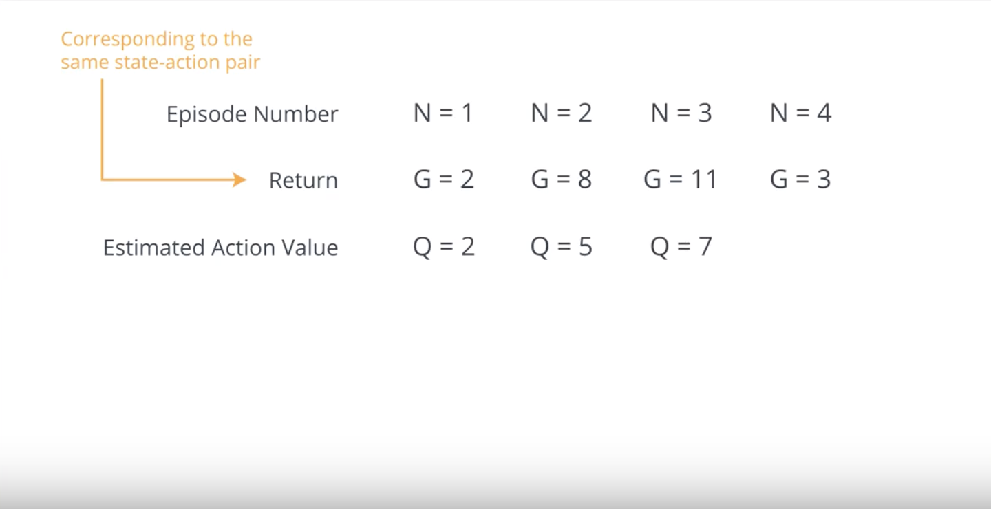
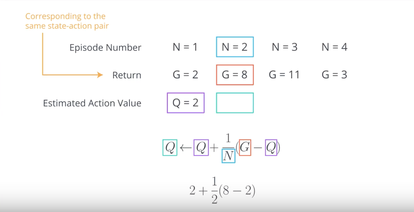
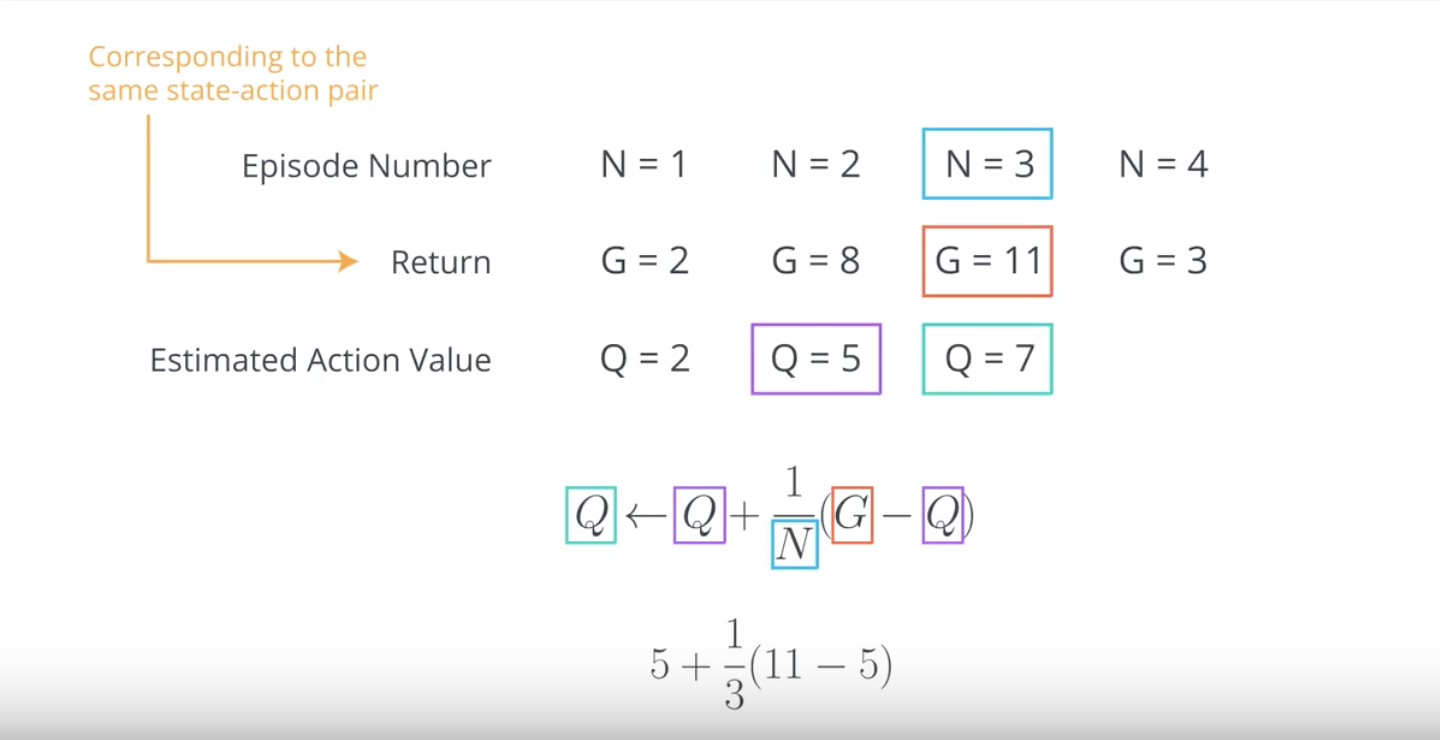
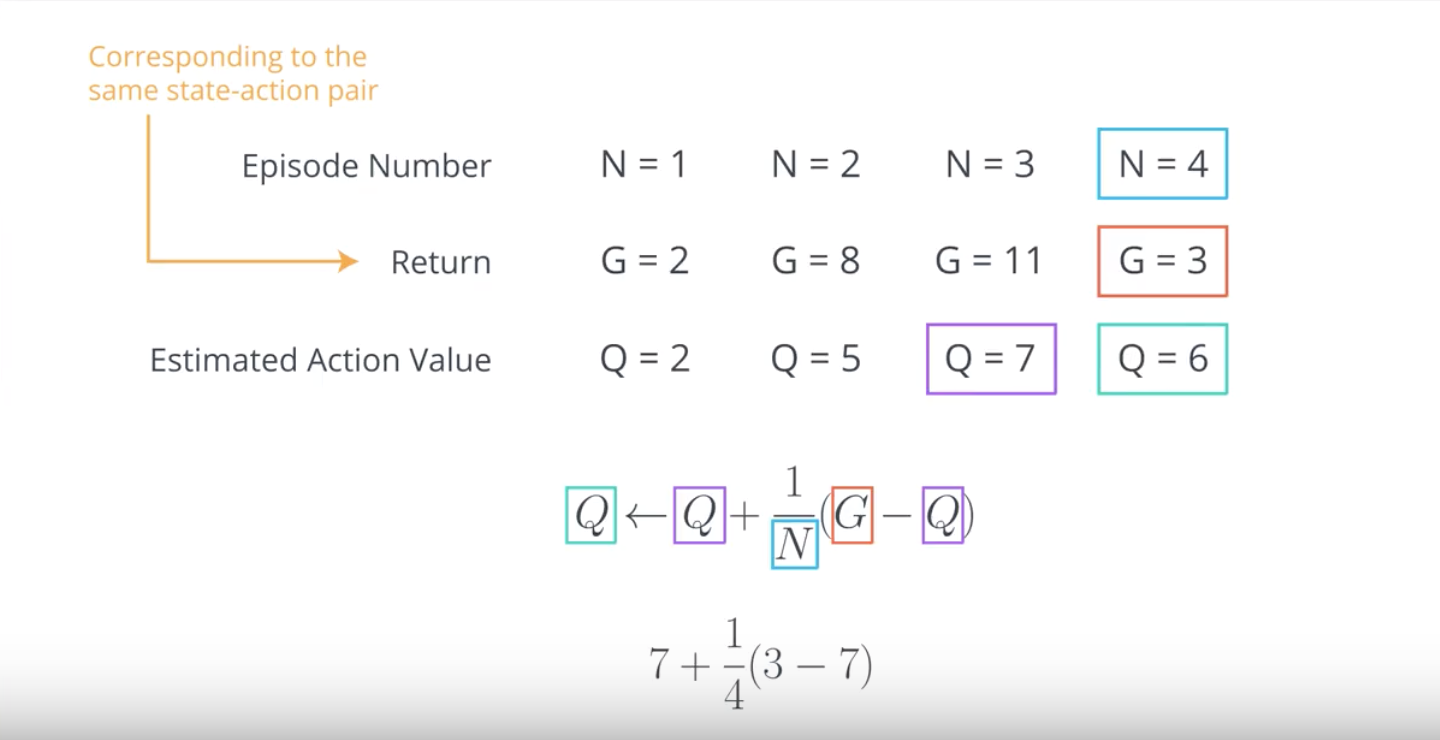
In our current algorithm for Monte Carlo control, we collect a large number of episodes to build the Q-table (as an estimate for the action-value function corresponding to the agent’s current policy). Then, after the values in the Q-table have converged, we use the table to come up with an improved policy.

Maybe it would be more efficient to update the Q-table after every episode. Then, the updated Q-table could be used to improve the policy. That new policy could then be used to generate the next episode, and so on.

from IPython.display import Image
Image(filename='./images/1-4-8-1_incremental_mean.png')

from IPython.display import Image
Image(filename='./images/1-4-8-2_before_applying_incremental_mean.png')

from IPython.display import Image
Image(filename='./images/1-4-8-3_incremental_mean.png')

from IPython.display import Image
Image(filename='./images/1-4-8-4_incremental_mean.png')

from IPython.display import Image
Image(filename='./images/1-4-8-5_incremental_mean.png')

from IPython.display import Image
Image(filename='./images/1-4-8-6_incremental_mean.png')

from IPython.display import Image
Image(filename='./images/1-4-8-7_incremental_mean.png')

from IPython.display import Image
Image(filename='./images/1-4-8-8_incremental_mean.png')

from IPython.display import Image
Image(filename='./images/1-4-8-9_incremental_mean.png')

from IPython.display import Image
Image(filename='./images/1-4-8-10_incremental_mean.png')

from IPython.display import Image
Image(filename='./images/1-4-8-11_incremental_mean.png')

In this case, even though we’re updating the policy before the values in the Q-table accurately approximate the action-value function, this lower-quality estimate nevertheless still has enough information to help us propose successively better policies. If you’re curious to learn more, you can read section 5.6 of the Sutton’s textbook.

Pseudocode

There are two relevant tables:

Q - Q-table, with a row for each state and a column for each action. The entry corresponding to state s and action a is denoted Q(s,a). N - table that keeps track of the number of first visits we have made to each state-action pair. The number of episodes the agent collects is equal to num_episodes.

from IPython.display import Image
Image(filename='./images/1-4-8-12_incremental_mean_pseudocode.png')

The algorithm proceeds by looping over the following steps:

• Step 1: The policy π is improved to be ϵ-greedy with respect to Q, and the agent uses π to collect an episode.
• Step 2: N is updated to count the total number of first visits to each state action pair.
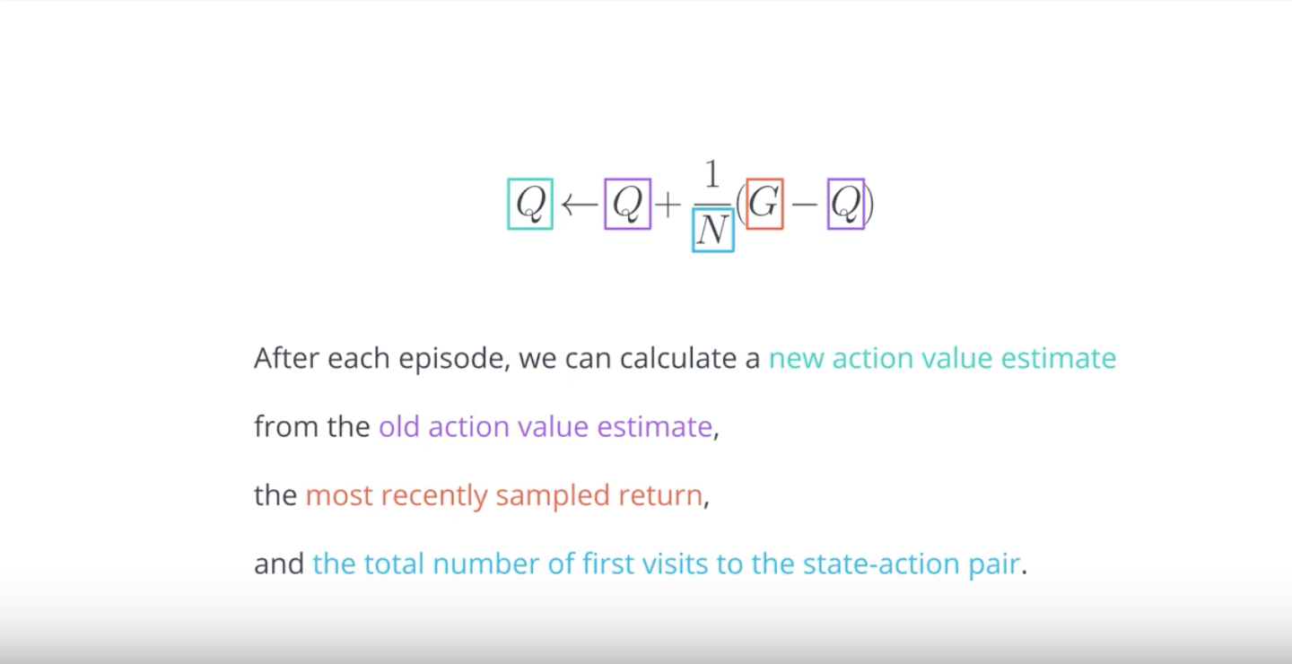
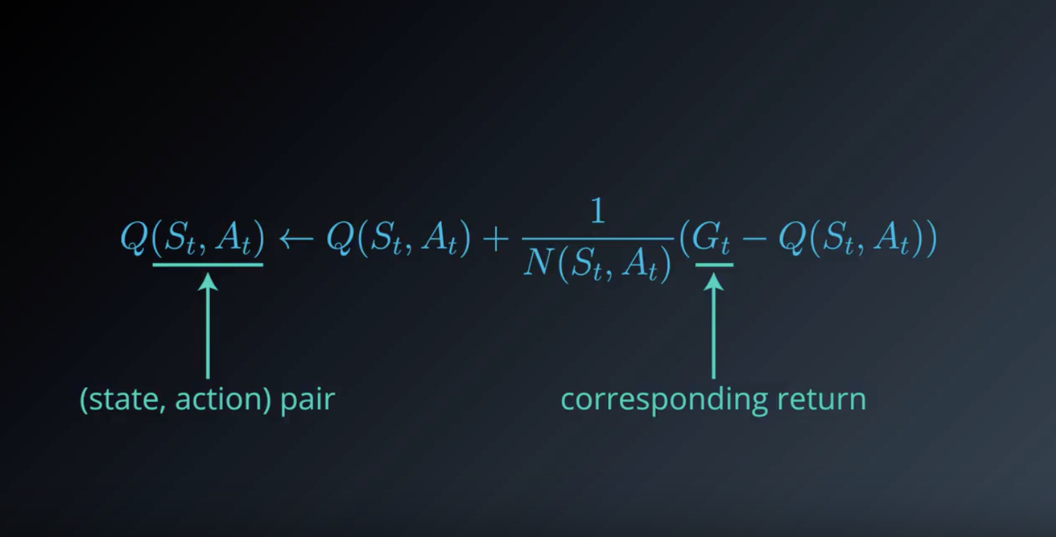
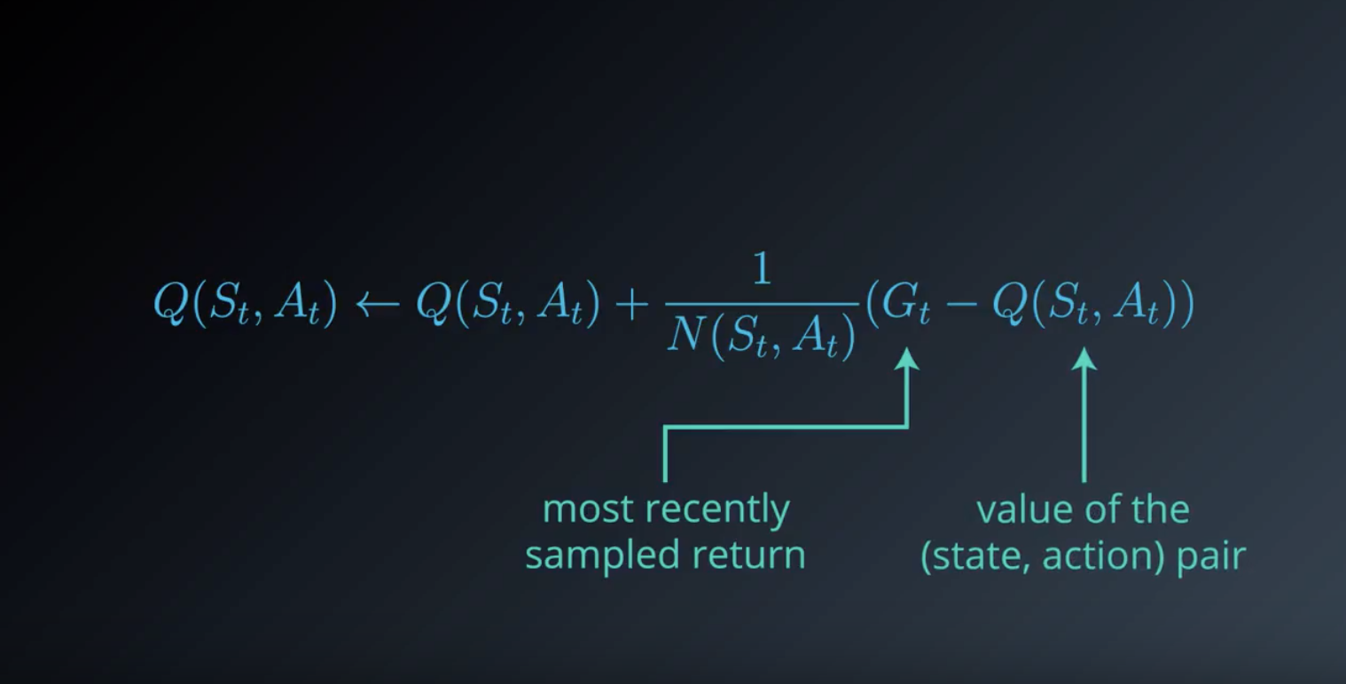
• Step 3: The estimates in Q are updated to take into account the most recent information.

In this way, the agent is able to improve the policy after every episode!

1-4-9 : Constant-alpha

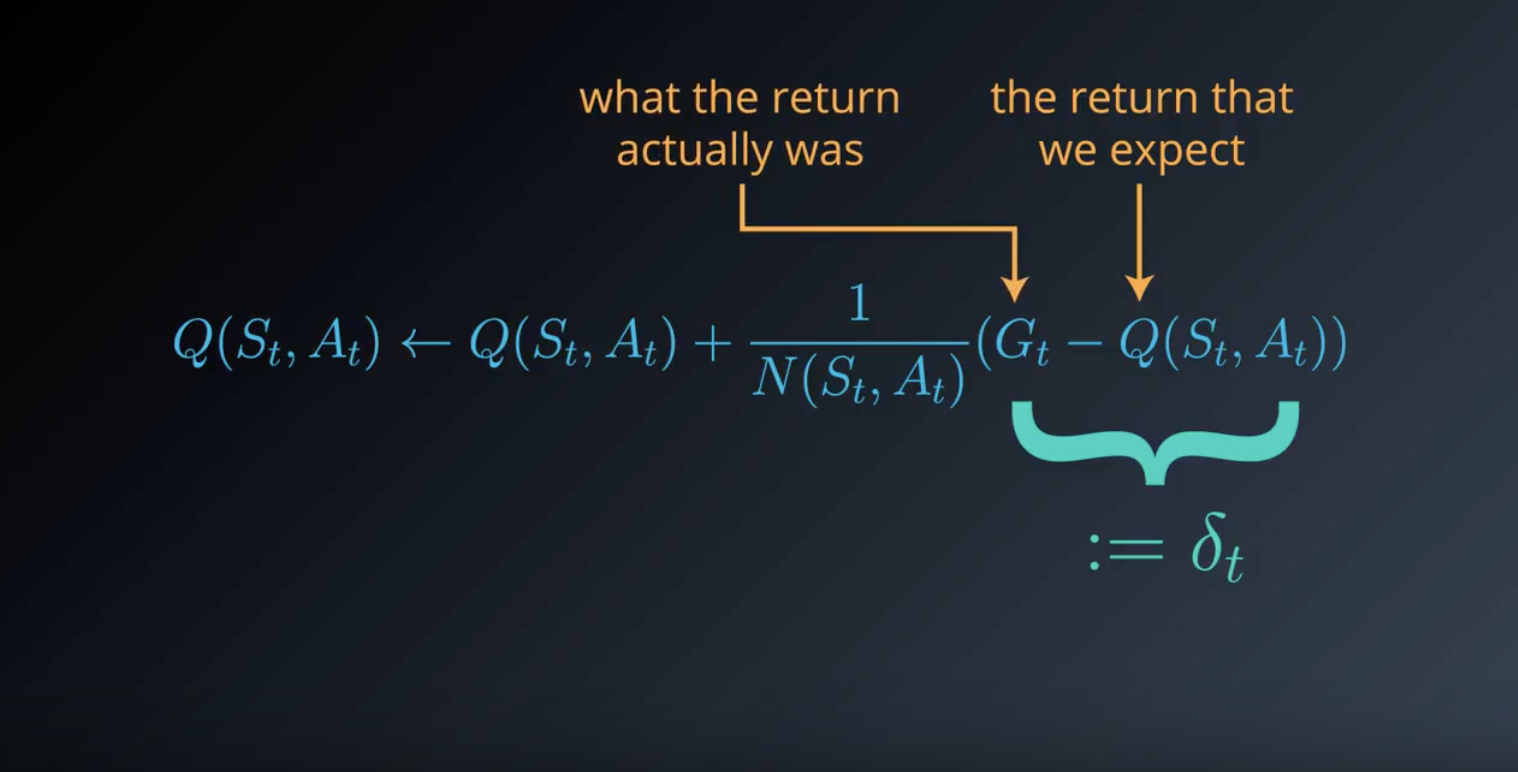
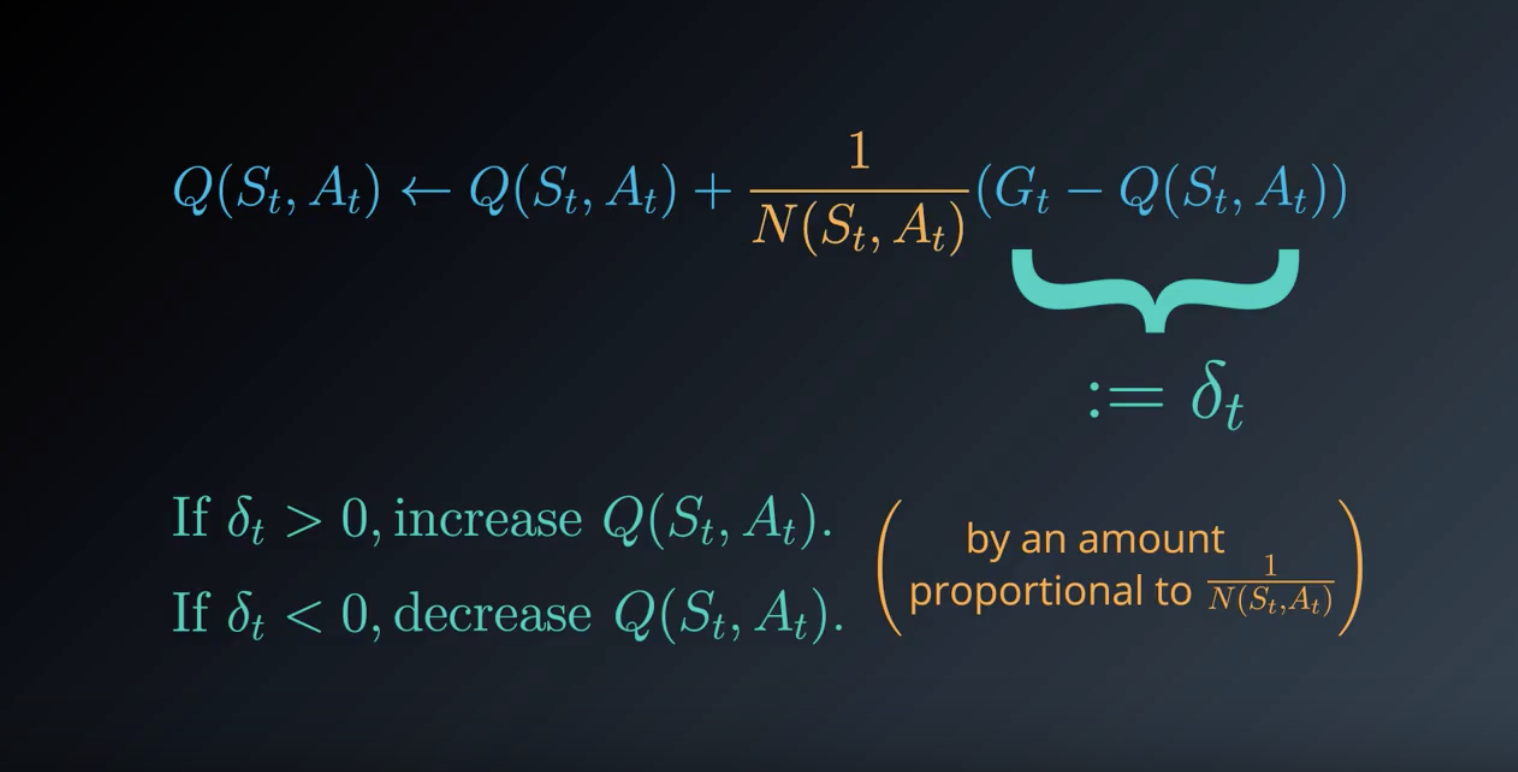
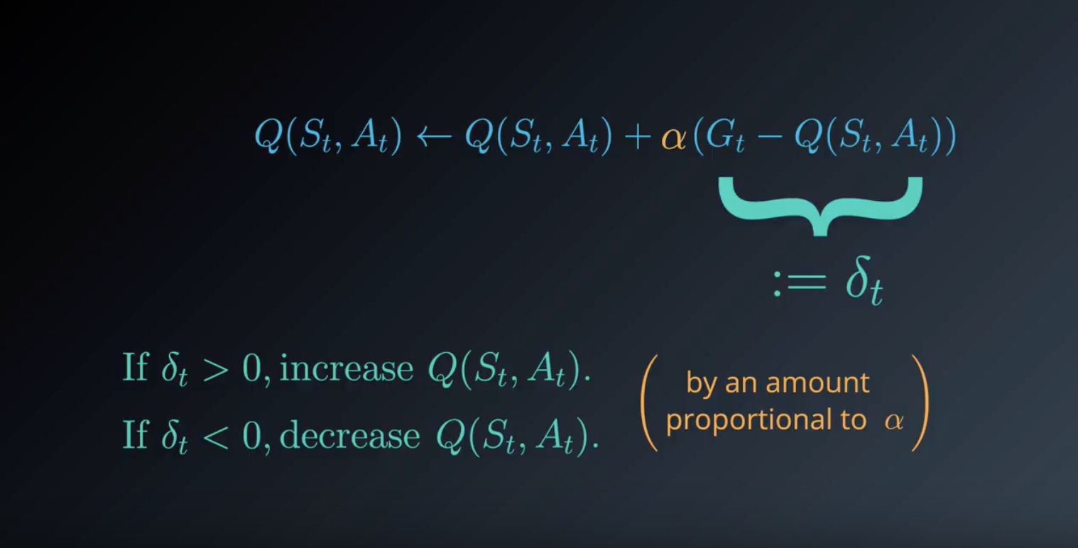
In the slides below, you will learn about another improvement that you can make to your Monte Carlo control algorithm.

from IPython.display import Image
Image(filename='./images/1-4-9-1_constant-alpha.png')

from IPython.display import Image
Image(filename='./images/1-4-9-2_constant-alpha.png')

from IPython.display import Image
Image(filename='./images/1-4-9-3_constant-alpha.png')

from IPython.display import Image
Image(filename='./images/1-4-9-4_constant-alpha.png')

from IPython.display import Image
Image(filename='./images/1-4-9-5_constant-alpha.png')

from IPython.display import Image
Image(filename='./images/1-4-9-6_constant-alpha.png')

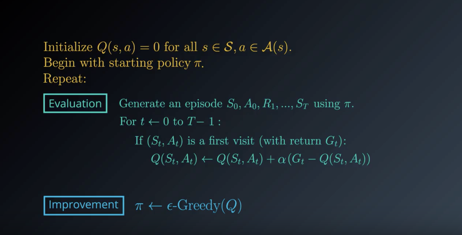
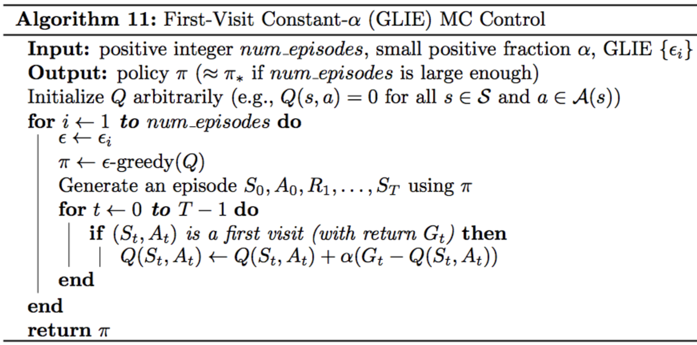
Pseudocode

The pseudocode for constant-α GLIE MC Control can be found below

from IPython.display import Image
Image(filename='./images/1-4-9-7_constant-alpha_pseudocode.png')

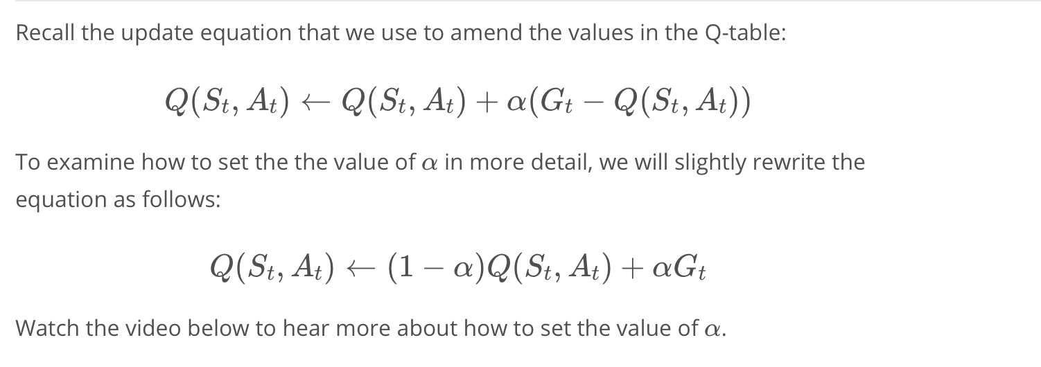
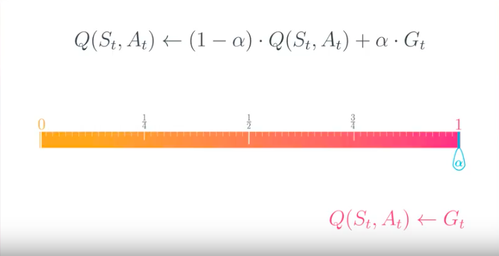
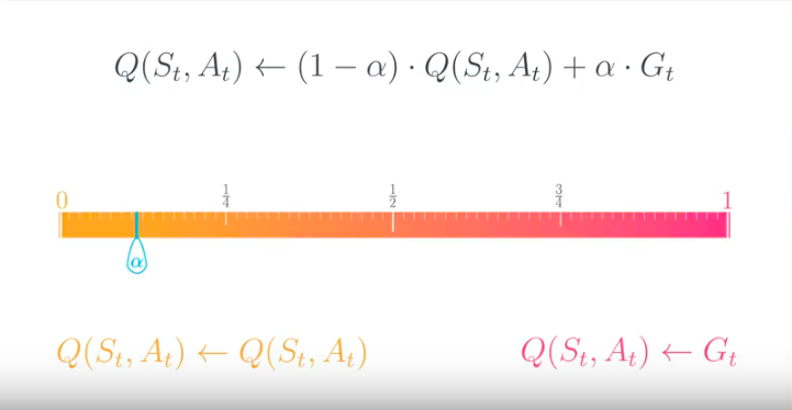
Setting the Value of α

from IPython.display import Image
Image(filename='./images/1-4-9-8_constant-alpha_setting.png')

from IPython.display import Image
Image(filename='./images/1-4-9-9_constant-alpha_is_1.png')

from IPython.display import Image
Image(filename='./images/1-4-9-10_constant-alpha_is_0.png')

from IPython.display import Image
Image(filename='./images/1-4-9-11_constant-alpha_should_be_set_between_0_and_1.png')

Here are some guiding principles that will help you to set the value of α when implementing constant-α MC control:

• You should always set the value for α to a number greater than zero and less than (or equal to) one.
  • If α=0, then the action-value function estimate is never updated by the agent.
  • If α=1, then the final value estimate for each state-action pair is always equal to the last return that was experienced by the agent (after visiting the pair).
• Smaller values for α encourage the agent to consider a longer history of returns when calculating the action-value function estimate. Increasing the value of α ensures that the agent focuses more on the most recently sampled returns.

Important Note:

When implementing constant-α MC control, you must be careful to not set the value of α too close to 1. This is because very large values can keep the algorithm from converging to the optimal policy π∗. However, you must also be careful to not set the value of α too low, as this can result in an agent who learns too slowly. The best value of α for your implementation will greatly depend on your environment and is best gauged through trial-and-error.